plottable
plottable draws a table as a matplotlib figure: every cell is an axes, so a
column can hold text, a bar or an image, and the finished table saves like any chart. sdvplot.plottable
adds two ColumnDefinition builders: logo_column draws each row's team as its logo or wordmark (any variant,
any season's mark) and headshot_column draws each row's player. sdvplot.team_colors supplies the colors for
team-tinted rows. The Tables cookbook shows one MLB table with logos; these five recipes cover the
WNBA, NFL, NHL, college football and men's college basketball, through sportsdataverse-py, and end with a
square image sized for a social post. Saved images go to a temporary folder.
import tempfile
from pathlib import Path

import matplotlib.pyplot as plt
import polars as pl
import sportsdataverse.cfb as cfb
import sportsdataverse.mbb as mbb
import sportsdataverse.nfl as nfl
import sportsdataverse.nhl as nhl
import sportsdataverse.wnba as wnba
from IPython.display import Image, display
from matplotlib import colormaps
from matplotlib.colors import LinearSegmentedColormap, to_rgba
from plottable import ColumnDefinition, Table
from plottable.cmap import normed_cmap
from plottable.plots import bar

import sdvplot
from sdvplot.plottable import headshot_column, logo_column

NFL_SEASON = 2025  # nflverse and cfbfastR name a season by the year it starts
SEASON = 2026  # the 2026 WNBA season and the 2025-26 NHL and men's college basketball seasons
OUT = Path(tempfile.mkdtemp())  # saved images go here, not into your working folder
1. Headshots and bars: the WNBA's leading scorers
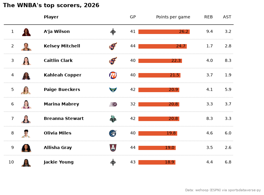
headshot_column draws each row's player from an ESPN athlete id, and logo_column draws the team beside the
name. The points column uses plottable's bar plot function, so each scoring average is a bar with its value
written next to it. ESPN files the All-Star Game and the Commissioner's Cup final under the regular season too, so the box scores
are first cut to the schedule's standard games, and the cell checks that no one played more games than a team's
schedule holds. The 2026 regular season's top ten scorers with 20 or more games:
# ESPN files the All-Star Game and the Commissioner's Cup final as regular-season games: keep the standard ones
schedule = wnba.load_wnba_schedule(seasons=[SEASON]).filter(
    (pl.col("season_type") == 2) & (pl.col("type_abbreviation") == "STD")
)
season_games = pl.concat([schedule["home_id"], schedule["away_id"]]).value_counts()["count"].max()
players = wnba.load_wnba_player_boxscore(seasons=[SEASON]).filter(
    pl.col("game_id").is_in(schedule["game_id"].implode()) & ~pl.col("did_not_play")
)
per_player = (
    players.sort("game_date")
    .group_by("athlete_id", "athlete_display_name", maintain_order=True)
    .agg(
        team=pl.col("team_abbreviation").last(),
        gp=pl.len(),
        ppg=pl.col("points").mean(),
        rpg=pl.col("rebounds").mean().round(1),
        apg=pl.col("assists").mean().round(1),
    )
)
assert per_player["gp"].max() <= season_games, "a player has more games than the schedule"
scorers = (
    per_player.filter(pl.col("gp") >= 20)
    .sort("ppg", descending=True)
    .head(10)
    .with_columns(rank=pl.int_range(1, 11))
    .select(
        "rank", photo="athlete_id", player="athlete_display_name", logo="team", gp="gp", ppg="ppg", rpg="rpg", apg="apg"
    )
    .to_pandas()
    .set_index("rank", drop=False)
)
fig, ax = plt.subplots(figsize=(10, 7))
Table(
    scorers,
    ax=ax,
    index_col="rank",
    column_definitions=[
        ColumnDefinition("rank", title="", width=0.3),
        headshot_column("photo", league="wnba", title="", width=0.6),
        ColumnDefinition("player", title="Player", width=1.8, textprops={"ha": "left", "weight": "bold"}),
        logo_column("logo", league="wnba", title="", width=0.5),
        ColumnDefinition("gp", title="GP", width=0.4),
        ColumnDefinition(
            "ppg",
            title="Points per game",
            width=1.6,
            plot_fn=bar,
            plot_kw={
                "xlim": (0, scorers["ppg"].max() * 1.1),
                "annotate": True,
                "color": "#e4572e",
                "height": 0.5,
                "formatter": "{:.1f}",
            },
        ),
        ColumnDefinition("rpg", title="REB", width=0.5),
        ColumnDefinition("apg", title="AST", width=0.5),
    ],
    row_divider_kw={"linewidth": 0.5, "linestyle": (0, (1, 3))},
)
ax.set_title(f"The WNBA's top scorers, {SEASON}", loc="left", fontweight="bold", fontsize=14)
fig.text(0.99, 0.01, "Data: wehoop (ESPN) via sportsdataverse-py", ha="right", fontsize=8, color="grey")
plt.show()
2. Wordmarks and color scales: NFL EPA
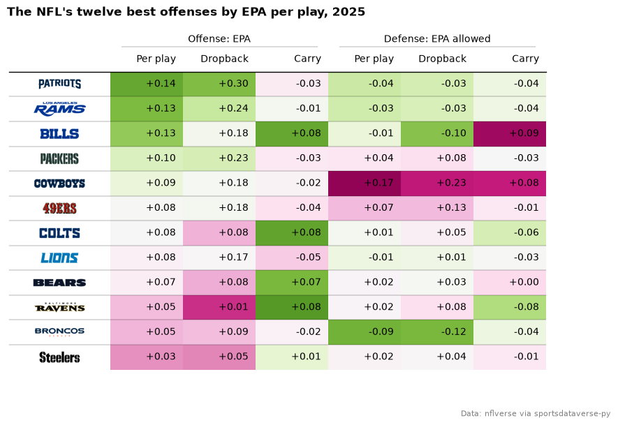
logo_column(mark_type="wordmark") draws the team's wordmark instead of its logo. The six EPA columns use
plottable's cmap with normed_cmap, which centers each column's color scale on its mean: green is good, so the
defensive columns take the reversed map. group= puts an Offense and a Defense header over their columns. The
twelve best teams of 2025 by EPA per play:
weeks = nfl.load_nfl_team_stats([NFL_SEASON]).filter(pl.col("season_type") == "REG")
dropbacks = pl.col("attempts") + pl.col("sacks_suffered")


def epa_rates(by):
    return weeks.group_by(team=by, maintain_order=True).agg(
        epa=(pl.col("passing_epa") + pl.col("rushing_epa")).sum() / (dropbacks + pl.col("carries")).sum(),
        pass_epa=pl.col("passing_epa").sum() / dropbacks.sum(),
        rush_epa=pl.col("rushing_epa").sum() / pl.col("carries").sum(),
    )


nfl_epa = (
    epa_rates(pl.col("team"))
    .join(epa_rates(pl.col("opponent_team")), on="team", suffix="_allowed")
    .sort("epa", descending=True)
    .head(12)
    .to_pandas()
    .set_index("team", drop=False)
)
good, bad = colormaps["PiYG"], colormaps["PiYG"].reversed()
labels = {"epa": "Per play", "pass_epa": "Dropback", "rush_epa": "Carry"}
fmt = "{:+.2f}"
fig, ax = plt.subplots(figsize=(10, 6.5))
Table(
    nfl_epa,
    ax=ax,
    index_col="team",
    column_definitions=[
        logo_column("team", league="nfl", mark_type="wordmark", title="", width=1.4),
        *[
            ColumnDefinition(
                c, title=labels[c], group="Offense: EPA", formatter=fmt, cmap=normed_cmap(nfl_epa[c], good)
            )
            for c in labels
        ],
        *[
            ColumnDefinition(
                f"{c}_allowed",
                title=labels[c],
                group="Defense: EPA allowed",
                formatter=fmt,
                cmap=normed_cmap(nfl_epa[f"{c}_allowed"], bad),
            )
            for c in labels
        ],
    ],
)
ax.set_title(f"The NFL's twelve best offenses by EPA per play, {NFL_SEASON}", loc="left", fontweight="bold")
fig.text(0.99, 0.01, "Data: nflverse via sportsdataverse-py", ha="right", fontsize=8, color="grey")
plt.show()
3. Team-colored rows and track bars: an NHL division
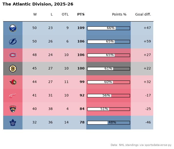
sdvplot.team_colors returns each team's primary color, and after the table is drawn every row's cells take that
color at a quarter opacity (table.rows[i].set_facecolor). The points-percentage column is a white bar over
an outlined track (plot_bg_bar) on a 0 to 100% scale. The Atlantic Division's final 2025-26 standings:
atlantic = (
    nhl.nhl_standings("2026-04-16")
    .filter(pl.col("division_name") == "Atlantic")
    .sort("points", descending=True)
    .select(
        logo="team_abbrev_default",
        w="wins",
        l="losses",
        otl="ot_losses",
        pts="points",
        pct="point_pctg",
        gd="goal_differential",
    )
    .to_pandas()
    .set_index("logo", drop=False)
)
fig, ax = plt.subplots(figsize=(8, 6.5))
table = Table(
    atlantic,
    ax=ax,
    index_col="logo",
    column_definitions=[
        logo_column("logo", league="nhl", title="", width=0.6),
        ColumnDefinition("w", title="W", width=0.5),
        ColumnDefinition("l", title="L", width=0.5),
        ColumnDefinition("otl", title="OTL", width=0.5),
        ColumnDefinition("pts", title="PTS", width=0.5, textprops={"weight": "bold"}),
        ColumnDefinition(
            "pct",
            title="Points %",
            width=1.4,
            plot_fn=bar,
            plot_kw={
                "xlim": (0, 1),
                "plot_bg_bar": True,
                "annotate": True,
                "color": "#ffffff",
                "height": 0.4,
                "formatter": "{:.0%}",
            },
        ),
        ColumnDefinition("gd", title="Goal diff.", width=0.7, formatter="{:+d}"),
    ],
    row_dividers=False,
)
for i, color in enumerate(sdvplot.team_colors("nhl", atlantic["logo"].tolist())):
    table.rows[i].set_facecolor(to_rgba(color, 0.25))
ax.set_title(f"The Atlantic Division, {SEASON - 1}-{SEASON % 100}", loc="left", fontweight="bold")
fig.text(0.99, 0.01, "Data: NHL standings via sportsdataverse-py", ha="right", fontsize=8, color="grey")
plt.show()
4. Logos from ESPN ids: college football ratings
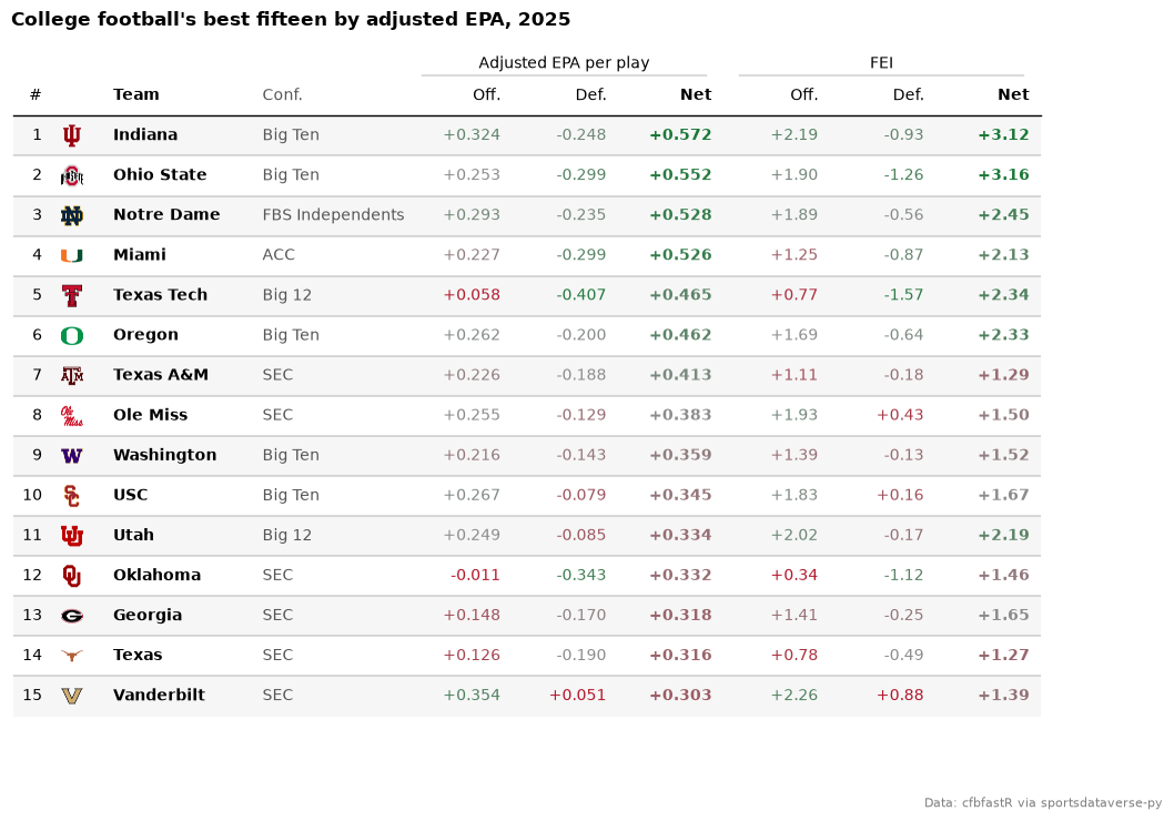
logo_column takes any id system sdvplot resolves; cfbfastR's ratings carry ESPN team ids, so the column reads
them with id_system="espn" and no name lookup. Two rating systems sit under their own group headers, each
column's text colored by its value (text_cmap with plottable's normed_cmap): green is good, red is
poor, and the defensive columns use the reversed scale because allowing less is better. The top fifteen of 2025 by net adjusted EPA per play:
summaries = cfb.load_cfb_team_summaries(NFL_SEASON).select("team_id", "pos_team", "conference")
ratings = cfb.load_cfb_ratings(NFL_SEASON)
assert summaries.schema["team_id"] == ratings.schema["team_id"]
top15 = (
    ratings.join(summaries, on="team_id")
    .sort("net_rank")
    .head(15)
    .select(
        "net_rank",
        logo="team_id",
        team="pos_team",
        conf="conference",
        off="adj_off_epa",
        dfn="adj_def_epa",
        net="adj_net",
        fei_off="fei_off",
        fei_def="fei_def",
        fei_net="fei_net",
    )
    .to_pandas()
    .set_index("net_rank", drop=False)
)
epa_fmt, fei_fmt = "{:+.3f}", "{:+.2f}"
good = LinearSegmentedColormap.from_list("good", ["#b2182b", "#8c8c8c", "#1a7837"])  # dark enough to read as text


def scale(column, cmap=good):
    """Color a column's text by its value, centered on its median."""
    return normed_cmap(top15[column], cmap=cmap, num_stds=2)


fig, ax = plt.subplots(figsize=(12, 8))
Table(
    top15,
    ax=ax,
    index_col="net_rank",
    column_definitions=[
        ColumnDefinition("net_rank", title="#", width=0.3),
        logo_column("logo", league="cfb", id_system="espn", title="", width=0.5),
        ColumnDefinition("team", title="Team", width=1.4, textprops={"ha": "left", "weight": "bold"}),
        ColumnDefinition("conf", title="Conf.", width=1.5, textprops={"ha": "left", "color": "#555555"}),
        ColumnDefinition("off", title="Off.", group="Adjusted EPA per play", formatter=epa_fmt, text_cmap=scale("off")),
        ColumnDefinition(
            "dfn",
            title="Def.",
            group="Adjusted EPA per play",
            formatter=epa_fmt,
            text_cmap=scale("dfn", good.reversed()),
        ),
        ColumnDefinition(
            "net",
            title="Net",
            group="Adjusted EPA per play",
            formatter=epa_fmt,
            text_cmap=scale("net"),
            textprops={"weight": "bold"},
        ),
        ColumnDefinition("fei_off", title="Off.", group="FEI", formatter=fei_fmt, text_cmap=scale("fei_off")),
        ColumnDefinition(
            "fei_def", title="Def.", group="FEI", formatter=fei_fmt, text_cmap=scale("fei_def", good.reversed())
        ),
        ColumnDefinition(
            "fei_net",
            title="Net",
            group="FEI",
            formatter=fei_fmt,
            text_cmap=scale("fei_net"),
            textprops={"weight": "bold"},
        ),
    ],
    even_row_color="#f6f6f6",
)
ax.set_title(f"College football's best fifteen by adjusted EPA, {NFL_SEASON}", loc="left", fontweight="bold")
fig.text(0.99, 0.01, "Data: cfbfastR via sportsdataverse-py", ha="right", fontsize=8, color="grey")
plt.show()
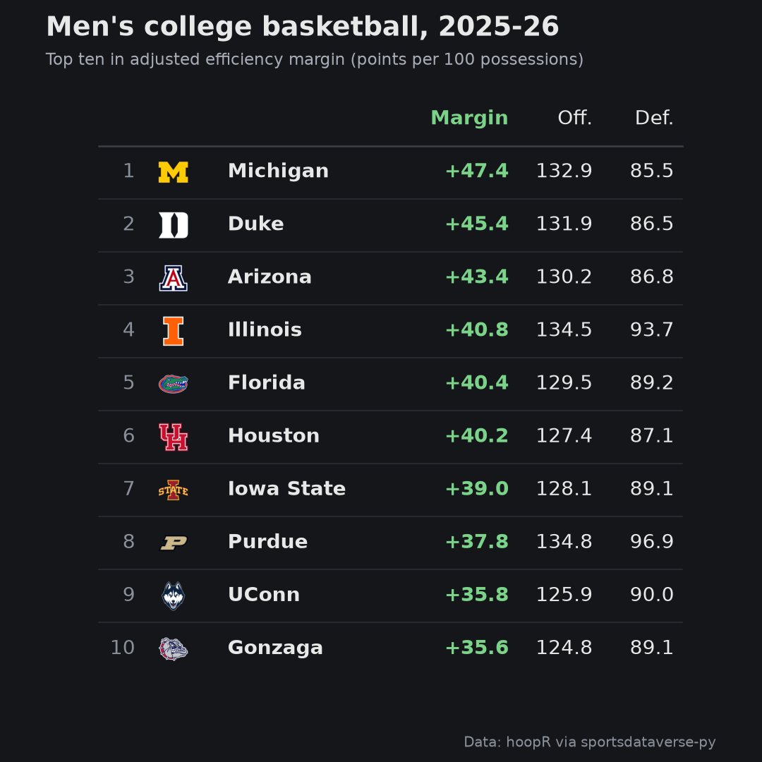
5. A square image for social: men's college basketball, dark
A social post wants a fixed pixel size, and a plottable table is a matplotlib figure, so the size is the figure's
inches times its dpi: 6 by 6 inches at 180 dpi is a 1080 by 1080 image. On a dark background logo_column's
variant="dark" uses the logos drawn for one. The 2025-26 top ten in adjusted efficiency margin, saved to a file
and shown from it:
names = mbb.load_mbb_team_boxscore(seasons=[SEASON]).select("team_id", "team_location").unique("team_id")
mbb_ratings = mbb.load_mbb_ratings(SEASON).with_columns(pl.col("team_id").cast(pl.Int32))  # ids ship as text here
assert names.schema["team_id"] == mbb_ratings.schema["team_id"]
top10 = (
    mbb_ratings.sort("rank")
    .head(10)
    .join(names, on="team_id", how="left")
    .select("rank", logo="team_id", team="team_location", em="adj_em", o="adj_o", d="adj_d")
    .to_pandas()
    .set_index("rank", drop=False)
)
BG, FG = "#14161a", "#e8e8e8"
fig, ax = plt.subplots(figsize=(6, 6), facecolor=BG)
ax.set_facecolor(BG)
Table(
    top10,
    ax=ax,
    index_col="rank",
    textprops={"color": FG, "fontsize": 11},
    column_definitions=[
        ColumnDefinition("rank", title="", width=0.3, textprops={"color": "#8a909a"}),
        logo_column("logo", league="mbb", id_system="espn", variant="dark", title="", width=0.5),
        ColumnDefinition("team", title="", width=1.5, textprops={"ha": "left", "weight": "bold"}),
        ColumnDefinition(
            "em", title="Margin", width=0.8, formatter="{:+.1f}", textprops={"color": "#7bd389", "weight": "bold"}
        ),
        ColumnDefinition("o", title="Off.", width=0.6, formatter="{:.1f}"),
        ColumnDefinition("d", title="Def.", width=0.6, formatter="{:.1f}"),
    ],
    col_label_divider_kw={"color": "#3a3f48"},
    row_divider_kw={"color": "#2c3038", "linewidth": 0.6},
)
fig.suptitle(
    f"Men's college basketball, {SEASON - 1}-{SEASON % 100}",
    x=0.06,
    ha="left",
    color=FG,
    fontweight="bold",
    fontsize=15,
)
fig.text(0.06, 0.915, "Top ten in adjusted efficiency margin (points per 100 possessions)", color="#a8adb7", fontsize=9)
fig.text(0.94, 0.02, "Data: hoopR via sportsdataverse-py", ha="right", fontsize=8, color="#8a909a")
path = OUT / "mbb_top10_square.png"
fig.savefig(path, dpi=180, facecolor=BG)
plt.close(fig)
print(plt.imread(path).shape[1::-1])
display(Image(filename=path, width=540))
(1080, 1080)
Run it yourself
Download the notebook (outputs cleared) or open it on GitHub.