pygal
pygal draws charts as SVG, with hover tooltips built in. sdvplot adds two things to it:
sdvplot.pygal.team_style() turns a list of teams into a pygal Style whose series colors are the team colors, and
add_logos / add_wordmarks / add_headshots place images on any XY-family chart (XY, DateLine,
DateTimeLine, ...) at the exact spot pygal draws each point. pygal writes axis labels as text, so there are no axis
logos; axis_logos raises a TypeError that says so.
The data is one completed season each from the NFL (nflverse), MLB (ESPN), the NBA and men's college basketball (hoopR), the WNBA (wehoop) and the NHL (fastRhockey), all through sportsdataverse-py.
import polars as pl
import pygal
import sportsdataverse.mbb as mbb
import sportsdataverse.mlb as mlb
import sportsdataverse.nba as nba
import sportsdataverse.nfl as nfl
import sportsdataverse.nhl as nhl
import sportsdataverse.wnba as wnba
from IPython.display import HTML, Image, display

import sdvplot
import sdvplot.pygal

NFL_SEASON = 2025  # football names a season by the year it starts
SEASON = 2026  # the 2026 MLB and WNBA seasons, and the 2025-26 NBA, NHL and college basketball season


def show_svg(chart):
    """Show a pygal chart inline as SVG (the logos are drawn while pygal renders)."""
    display(HTML(chart.render(is_unicode=True, disable_xml_declaration=True)))


def pad(values, share=0.08):
    """An axis range with room at both ends, so the logos at the edges are not cut off."""
    lo, hi = min(values), max(values)
    return lo - (hi - lo) * share, hi + (hi - lo) * share
pygal's own notebook display is a PNG through cairosvg; show_svg keeps the chart as SVG so its tooltips work.
Every chart below renders with the logos, because sdvplot hooks into pygal's render step rather than editing one
finished SVG.
1. A scatter with team logos
A pygal scatter is an XY chart with stroke=False. Give each point a label so pygal's tooltip names the team,
then call add_logos with the same x and y. NFL offense against defense, EPA per play:
weeks = nfl.load_nfl_team_stats([NFL_SEASON]).filter(pl.col("season_type") == "REG")
plays = pl.col("attempts") + pl.col("sacks_suffered") + pl.col("carries")
epa = pl.col("passing_epa") + pl.col("rushing_epa")
nfl_epa = (
    weeks.group_by("team", maintain_order=True)
    .agg(off_epa=epa.sum() / plays.sum())
    .join(
        weeks.group_by(team=pl.col("opponent_team"), maintain_order=True).agg(def_epa=epa.sum() / plays.sum()),
        on="team",
    )
    .sort("team")
)

chart = pygal.XY(
    stroke=False, width=800, height=560, dots_size=3, show_legend=False,
    xrange=pad(nfl_epa["off_epa"]), range=pad(nfl_epa["def_epa"]),
    title=f"NFL EPA per play, {NFL_SEASON} regular season (lower defense EPA is better)",
    x_title="Offense EPA per play", y_title="Defense EPA per play allowed",
)  # fmt: skip
chart.add("teams", [{"value": (o, d), "label": t} for t, o, d in nfl_epa.iter_rows()])
sdvplot.add_logos(chart, nfl_epa["off_epa"], nfl_epa["def_epa"], nfl_epa["team"], league="nfl", height=0.08)
show_svg(chart)
2. Wordmarks instead of logos
add_wordmarks takes the same arguments as add_logos. A wordmark is wider than it is tall, so a smaller height
keeps neighbours apart, and a wordmark with a lot of empty space around its letters draws small. MLB runs scored and allowed per game:
mlb_runs = (
    mlb.espn_mlb_standings(season=SEASON)
    .with_columns(
        rs=pl.col("points_for") / pl.col("games_played"), ra=pl.col("points_against") / pl.col("games_played")
    )
    .sort("team_abbreviation")
)

chart = pygal.XY(
    stroke=False, width=800, height=560, dots_size=2, show_legend=False,
    xrange=pad(mlb_runs["rs"]), range=pad(mlb_runs["ra"]),
    title=f"MLB runs scored and allowed per game, {SEASON}", x_title="Runs scored per game",
    y_title="Runs allowed per game",
)  # fmt: skip
chart.add(
    "teams", [{"value": (s, a), "label": t} for t, s, a in mlb_runs.select("team_abbreviation", "rs", "ra").iter_rows()]
)
sdvplot.add_wordmarks(chart, mlb_runs["rs"], mlb_runs["ra"], mlb_runs["team_abbreviation"], league="mlb", height=0.07)
show_svg(chart)
3. Team colors on a bar chart
team_style() works on every pygal chart, not only XY: it returns a Style whose colors follow the order you add
the series. Add one series per team and each bar takes its team's primary color; a label on each value and
print_labels=True write the team on its bar. The ten NBA teams that took the most threes per game:
nba_threes = (
    nba.load_nba_team_boxscore(seasons=[SEASON])
    .filter(pl.col("season_type") == 2)
    .group_by("team_id", "team_abbreviation", maintain_order=True)
    .agg(games=pl.len(), fg3a=pl.col("three_point_field_goals_attempted").mean())
    .filter(pl.col("games") > 10)
    .with_columns(pl.col("team_id").cast(pl.Int64).cast(pl.Utf8))
    .sort("fg3a", descending=True)
    .head(10)
)

style = sdvplot.pygal.team_style(nba_threes["team_id"], league="nba", font_family="sans-serif")
chart = pygal.Bar(
    style=style, width=800, height=480, show_legend=False, print_labels=True,
    title=f"NBA three-point attempts per game, {SEASON - 1}-{SEASON % 100} (top 10)", y_title="3PA per game",
)  # fmt: skip
for team, fg3a in nba_threes.select("team_abbreviation", "fg3a").iter_rows():
    chart.add(team, [{"value": round(fg3a, 1), "label": team}])
show_svg(chart)
4. Player headshots
add_headshots places ESPN headshots by athlete id. WNBA scoring leaders, points per game against minutes per
game (players with at least 20 games):
# ESPN files the All-Star Game and the Commissioner's Cup final as regular-season games: keep the standard ones
schedule = wnba.load_wnba_schedule(seasons=[SEASON]).filter(
    (pl.col("season_type") == 2) & (pl.col("type_abbreviation") == "STD")
)
season_games = pl.concat([schedule["home_id"], schedule["away_id"]]).value_counts()["count"].max()
per_player = (
    wnba.load_wnba_player_boxscore(seasons=[SEASON])
    .filter(
        pl.col("game_id").is_in(schedule["game_id"].implode())
        & pl.col("did_not_play").not_()
        & pl.col("minutes").is_not_null()
    )
    .group_by("athlete_id", "athlete_display_name", maintain_order=True)
    .agg(games=pl.len(), mpg=pl.col("minutes").mean(), ppg=pl.col("points").mean())
)
assert per_player["games"].max() <= season_games, "a player has more games than the schedule"
wnba_players = (
    per_player.filter(pl.col("games") >= 20)
    .sort("ppg", descending=True)
    .head(12)
    .with_columns(pl.col("athlete_id").cast(pl.Int64).cast(pl.Utf8))
)

chart = pygal.XY(
    stroke=False, width=800, height=560, dots_size=2, show_legend=False,
    xrange=pad(wnba_players["mpg"]), range=pad(wnba_players["ppg"], 0.12),
    title=f"WNBA scoring leaders, {SEASON}", x_title="Minutes per game", y_title="Points per game",
)  # fmt: skip
chart.add(
    "players",
    [
        {"value": (m, p), "label": n}
        for n, m, p in wnba_players.select("athlete_display_name", "mpg", "ppg").iter_rows()
    ],
)
sdvplot.add_headshots(
    chart, wnba_players["mpg"], wnba_players["ppg"], wnba_players["athlete_id"], league="wnba", height=0.1
)
show_svg(chart)
5. A date line: team colors and a logo at the end of each line
DateLine is in the XY family, so the logos take dates for x. Here team_style() colors the lines and
add_logos marks where each team finished. Cumulative wins in the standard games
of the schedule above, for four WNBA teams spread evenly from the top of the standings to the bottom:
wnba_games = (
    wnba.load_wnba_team_boxscore(seasons=[SEASON])
    .filter(pl.col("game_id").is_in(schedule["game_id"].implode()))
    .sort("game_date")
    .with_columns(wins=pl.col("team_winner").cast(pl.Int64).cum_sum().over("team_abbreviation"))
)
standings = (
    wnba_games.group_by("team_abbreviation")
    .agg(pl.col("wins").max())
    .sort(["wins", "team_abbreviation"], descending=[True, False])
)["team_abbreviation"]
n = standings.len()
leaders = standings.gather([round(i * (n - 1) / 3) for i in range(4)]).to_list()  # first, last and two between
ends_max = wnba_games["wins"].max()

chart = pygal.DateLine(
    style=sdvplot.pygal.team_style(leaders, league="wnba"), width=800, height=480, dots_size=2,
    x_label_rotation=25, legend_at_bottom=True, range=(0, ends_max * 1.12), y_title="Wins",
    title=f"WNBA cumulative wins, {SEASON}",
)  # fmt: skip
ends = []
for team in leaders:
    rows = wnba_games.filter(pl.col("team_abbreviation") == team).select("game_date", "wins")
    chart.add(team, list(rows.iter_rows()))
    ends.append(rows.row(-1))
sdvplot.add_logos(chart, [d for d, _ in ends], [w for _, w in ends], leaders, league="wnba", height=0.09)
show_svg(chart)
6. A dark chart with dark-background logos
team_style() passes any other Style option through, so one call sets the team colors and a dark background.
variant="dark" picks each team's logo drawn for dark backgrounds. NHL goals for and against per game, with each
team its own series so its dot takes its secondary color (the logos name the teams, so the legend is off):
nhl_teams = (
    nhl.load_nhl_team_box(seasons=[SEASON])
    .filter(pl.col("game_id") // 10_000 % 100 == 2)
    .group_by("team_abbrev", maintain_order=True)
    .agg(gf=pl.col("goals").mean(), ga=pl.col("goals_against").mean())
    .sort("team_abbrev")
)

dark = sdvplot.pygal.team_style(
    nhl_teams["team_abbrev"], league="nhl", which="secondary", background="#15171c", plot_background="#15171c",
    foreground="#d6d8de", foreground_strong="#ffffff", foreground_subtle="#3a3e48",
)  # fmt: skip
chart = pygal.XY(
    style=dark, stroke=False, width=800, height=560, dots_size=4, show_legend=False,
    xrange=pad(nhl_teams["gf"]), range=pad(nhl_teams["ga"]),
    title=f"NHL goals for and against per game, {SEASON - 1}-{SEASON % 100}", x_title="Goals for per game",
    y_title="Goals against per game", inverse_y_axis=True,
)  # fmt: skip
for team, gf, ga in nhl_teams.iter_rows():
    chart.add(team, [(gf, ga)])
sdvplot.add_logos(
    chart, nhl_teams["gf"], nhl_teams["ga"], nhl_teams["team_abbrev"], league="nhl", variant="dark", height=0.07
)
show_svg(chart)
7. Export a PNG
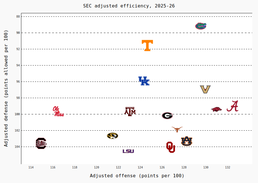
pygal's render_to_png() rasterizes the SVG with cairosvg. cairosvg does not fetch linked images, so pass
embed=True: sdvplot puts each logo in the SVG as a data URI and the PNG needs no network. The SEC's adjusted
offensive and defensive efficiency:
sec = (
    mbb.load_mbb_ratings(SEASON)
    .join(
        sdvplot.teams("mbb").filter(pl.col("conference") == "Southeastern Conference").select("team_id", "name"),
        on="team_id",
    )
    .sort("team_id")
)

chart = pygal.XY(
    stroke=False, width=900, height=640, dots_size=2, show_legend=False,
    xrange=pad(sec["adj_o"]), range=pad(sec["adj_d"]),
    title=f"SEC adjusted efficiency, {SEASON - 1}-{SEASON % 100}", x_title="Adjusted offense (points per 100)",
    y_title="Adjusted defense (points allowed per 100)", inverse_y_axis=True,
)  # fmt: skip
chart.add("teams", [{"value": (o, d), "label": n} for n, o, d in sec.select("name", "adj_o", "adj_d").iter_rows()])
sdvplot.add_logos(
    chart, sec["adj_o"], sec["adj_d"], sec["team_id"], league="mbb", season=SEASON, height=0.08, embed=True
)
display(Image(data=chart.render_to_png(dpi=144), width=760))
Run it yourself
Download the notebook (outputs cleared) or open it on GitHub.