College hoops tiers
The brief: a college basketball account wants an end-of-season Big Ten tier list, the kind fans argue about,
but backed by a power rating instead of vibes, as a 1080 x 1080 post plus a 1200 x 675 cut. The rating is
SportsDataverse's adjusted efficiency margin for men's college basketball through sportsdataverse.mbb, and
team_tiers (sdvplot's port of sdvplotR's Tiermaker) draws the list.
import tempfile
from pathlib import Path

import matplotlib.pyplot as plt
import polars as pl
import sportsdataverse.mbb as mbb
from IPython.display import Image
from PIL import Image as PILImage

import sdvplot
from sdvplot.matplotlib import team_tiers

SEASON = 2026  # the 2025-26 season, named by the year it ends
CONFERENCE = "Big Ten Conference"
OUT = Path(tempfile.mkdtemp(prefix="sdvplot-recipe-"))  # where the exports go; use your own folder
1. Get the data
One row per team: adjusted offense, defense and their margin (points per 100 possessions better than an average Division I team, adjusted for opponents). The ratings carry ESPN team ids; sdvplot's team table supplies each team's conference and abbreviation for the same ids.
ratings = mbb.load_mbb_ratings(SEASON)
teams = sdvplot.teams("mbb").select("team_id", "abbr", "short_name", "conference")
assert ratings.schema["team_id"] == teams.schema["team_id"]  # ESPN ids as strings on both sides
league = (
    ratings.join(teams, on="team_id")
    .filter(pl.col("conference") == CONFERENCE)
    .sort("adj_em", descending=True)
    .select("team_id", "abbr", "short_name", "rank", "adj_em")
)
league
| team_id | abbr | short_name | rank | adj_em |
|---|---|---|---|---|
| 130 | MICH | Michigan | 1 | 47.352765 |
| 356 | ILL | Illinois | 4 | 40.779914 |
| 2509 | PUR | Purdue | 8 | 37.843323 |
| 127 | MSU | Michigan St | 11 | 35.216251 |
| 158 | NEB | Nebraska | 17 | 32.265985 |
| … | … | … | … | … |
| 135 | MINN | Minnesota | 78 | 15.001971 |
| 2483 | ORE | Oregon | 92 | 12.254012 |
| 120 | MD | Maryland | 121 | 7.168668 |
| 164 | RUTG | Rutgers | 124 | 6.900419 |
| 213 | PSU | Penn State | 130 | 6.3738 |
2. The first draft
Five tiers of equal size, straight into team_tiers.
equal = pl.int_range(pl.len()) * 5 // pl.len() + 1  # five tiers of (nearly) equal size
draft = league.select(team="team_id", tier_no=equal)
fig = team_tiers(draft, "mbb")
plt.show()
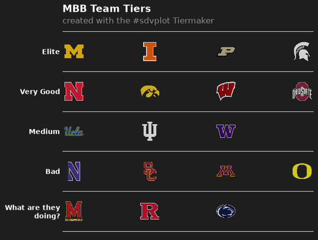
It looks like a tier list, but the tiers are wrong. Equal-sized groups put Michigan, the best team in the country, in the same tier as teams more than ten points worse per 100 possessions, and split neighbors who are barely a point apart. The default labels ("Elite" ... "What are they doing?") are jokes, not information.
3. Let the ratings draw the lines
Tiers should break where the ratings do. Sorting by rating and measuring the gap to the team above makes the widest gaps easy to find; cutting at the four widest gives five tiers whose members are close to each other.
league = league.with_columns(gap=pl.col("adj_em").shift(1) - pl.col("adj_em"))
cut = league["gap"].drop_nulls().sort(descending=True)[3]  # the fourth-widest gap
league = league.with_columns(tier_no=(pl.col("gap").fill_null(0) >= cut).cum_sum() + 1)
league.filter(pl.col("gap") >= cut).select("short_name", "adj_em", "gap", "tier_no")
| short_name | adj_em | gap | tier_no |
|---|---|---|---|
| Illinois | 40.779914 | 6.572851 | 2 |
| Washington | 20.961117 | 3.22975 | 3 |
| USC | 15.505063 | 3.014913 | 4 |
| Maryland | 7.168668 | 5.085345 | 5 |
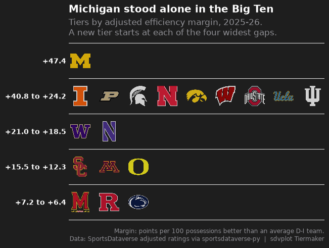
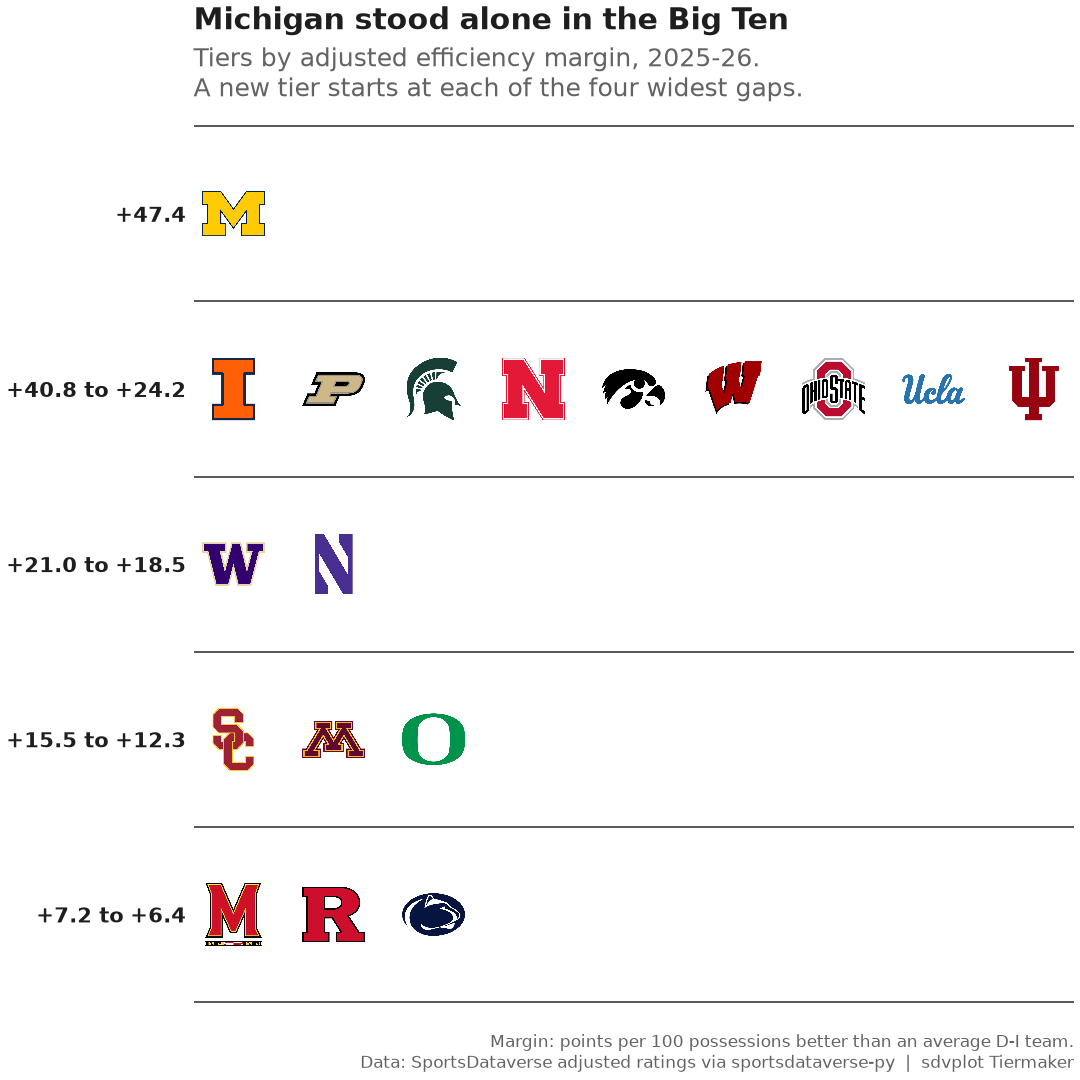
Each row above starts a new tier: Michigan stands alone, and the gaps at the top (6.6 points) and near the bottom (5.1) are the conference's real dividing lines.
4. Labels that say something
Each tier's label becomes the rating range of its members, so the list carries its own evidence, and the title states
the finding. tier_rank keeps teams in rating order inside a tier. The subtitle explains the rating and the rule for
the cuts; the caption names the data.
tiers = (
    league.group_by("tier_no", maintain_order=True)
    .agg(lo=pl.col("adj_em").min(), hi=pl.col("adj_em").max())
    .sort("tier_no")
)
tier_desc = {
    row["tier_no"]: f"{row['hi']:+.1f}" if row["lo"] == row["hi"] else f"{row['hi']:+.1f} to {row['lo']:+.1f}"
    for row in tiers.iter_rows(named=True)
}
best = league.row(0, named=True)
data = league.select(team="team_id", tier_no="tier_no", tier_rank=pl.int_range(1, pl.len() + 1).over("tier_no"))


def tier_list(height=0.12, alpha=0.8, theme="dark"):
    return team_tiers(
        data,
        "mbb",
        title=f"{best['short_name']} stood alone in the Big Ten",
        subtitle=f"Tiers by adjusted efficiency margin, {SEASON - 1}-{SEASON % 100:02d}.\n"
        "A new tier starts at each of the four widest gaps.",
        caption="Margin: points per 100 possessions better than an average D-I team.\n"
        "Data: SportsDataverse adjusted ratings via sportsdataverse-py  |  sdvplot Tiermaker",
        tier_desc=tier_desc,
        height=height,
        alpha=alpha,
        theme=theme,
    )


fig = tier_list()
plt.show()
5. Light or dark
On the dark Tiermaker background, team_tiers draws each school's dark-background logo (its default
variant="auto"), so Iowa's hawk is gold, Michigan State's Spartan white and Penn State's lion outlined instead of
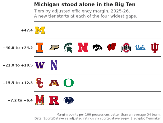
fading into the background. A light background suits a page or feed that is white anyway: theme="light" draws the
tiers on white with dark labels and lines, and each school's usual logo. The logos go to full opacity too
(alpha=1); the default 0.8 softens them against the dark background but washes them out on white. The exports
below use the light one.
fig = tier_list(alpha=1, theme="light")
plt.show()
6. Export at social sizes
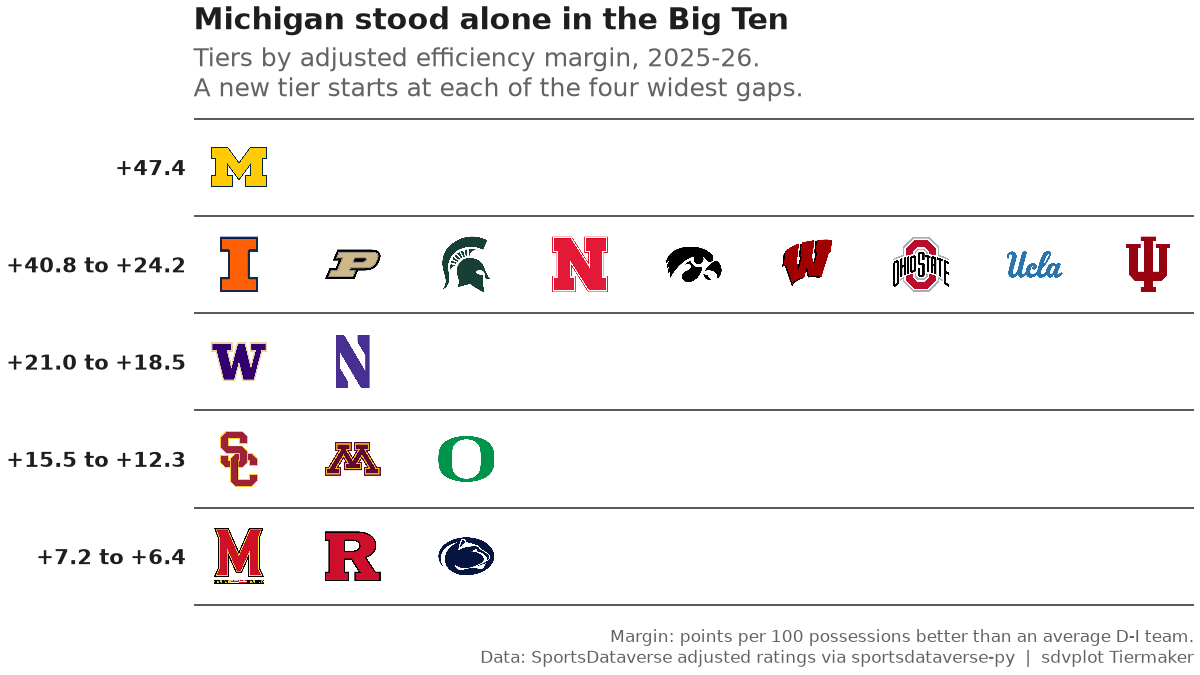
team_tiers returns an ordinary matplotlib figure with constrained layout, so set_size_inches re-lays it at each
export size. The logos are a fraction of the panel's height, and the square's panel is taller but narrower than the
wide cut's, so nine logos in one tier would collide there: the square gets a smaller height. Nine teams in a row
is also why the wide 1200 x 675 cut is the better post here.
exports = {"big_ten_tiers_1200x675.png": ((8, 4.5), 0.12), "big_ten_tiers_1080x1080.png": ((7.2, 7.2), 0.075)}
for name, (size, height) in exports.items():
    fig = tier_list(height, alpha=1, theme="light")
    fig.set_size_inches(*size)
    fig.savefig(OUT / name, dpi=150)
    plt.close(fig)
    print(name, PILImage.open(OUT / name).size)
Image(OUT / "big_ten_tiers_1200x675.png", width=700)
big_ten_tiers_1200x675.png (1200, 675)
big_ten_tiers_1080x1080.png (1080, 1080)
The 1080 x 1080 cut:
Image(OUT / "big_ten_tiers_1080x1080.png", width=540)
Run it yourself
Download the notebook (outputs cleared) or open it on GitHub.