Surfaces and shot charts

Nine recipes for playing surfaces and the charts drawn on them: surface() for every sport it supports, team colors and a center logo, NBA and WNBA shot charts from the stats-API shot files (converted with court_coords), a vertical half court, a hockey goal map, a baseball field and a soccer shot map on an mplsoccer pitch. Surfaces are drawn by sportypy. The data is one season each from the NFL (nflverse), the NBA, WNBA and college basketball (hoopR, wehoop and the stats-API shot files the SportsDataverse publishes on GitHub), the NHL (fastRhockey) and the Premier League (ESPN), all through sportsdataverse-py; nothing calls stats.nba.com.

import logging

import matplotlib.pyplot as plt
import polars as pl
import sportsdataverse.mbb as mbb
import sportsdataverse.nba as nba
import sportsdataverse.nfl as nfl
import sportsdataverse.nhl as nhl
import sportsdataverse.soccer as soccer
import sportsdataverse.wbb as wbb
import sportsdataverse.wnba as wnba

import sdvplot

# sportypy's football fields ask for the Clarendon font; where it is not installed, matplotlib logs one line per
# yard number and draws them in its default font. Quiet that log.
logging.getLogger("matplotlib.font_manager").setLevel(logging.ERROR)
NFL_SEASON = 2025  # nflverse names a season by the year it starts
SEASON = 2026  # the 2026 WNBA season and the 2025-26 NBA, NHL and college basketball season

1. Every surface sdvplot can draw

surface(league, team) picks sportypy's surface for the league and paints it in the team's colors where the sport has team-colored parts: end zones, the lane and apron, the center line and boards. Baseball fields and soccer pitches have none, so the team is left out there. (The WNBA and college courts are in recipe 3.)

examples = [
    ("nfl", "SEA", "NFL: Seattle"),
    ("cfb", "84", "College football: Indiana"),
    ("nba", "OKC", "NBA: Oklahoma City"),
    ("nhl", "COL", "NHL: Colorado"),
    ("mlb", None, "MLB"),
    ("soccer", None, "Soccer"),
]
fig, axes = plt.subplots(2, 3, figsize=(10, 5.5))
for ax, (league, team, label) in zip(axes.flat, examples, strict=True):
    sdvplot.surface(league, team, ax=ax)
    ax.set_title(label, fontsize=9)
fig.suptitle("sdvplot.surface(): one call per league", x=0.01, ha="left", fontweight="bold")
plt.show()

The college team is an ESPN id (84 is Indiana) and the pros are abbreviations; any value resolve understands works.

2. The champion's field, with a logo at midfield

center_logo=True puts the team's logo at the center of the surface (a quarter of the Axes tall); a number sets another height. The Super Bowl winner, read from nflverse's schedule:

sb = nfl.load_nfl_schedule([NFL_SEASON]).filter(pl.col("game_type") == "SB").row(0, named=True)
home_won = sb["home_score"] > sb["away_score"]
winner, loser = (sb["home_team"], sb["away_team"]) if home_won else (sb["away_team"], sb["home_team"])
score = f"{max(sb['home_score'], sb['away_score'])}-{min(sb['home_score'], sb['away_score'])}"

fig, ax = plt.subplots(figsize=(8.5, 5))
sdvplot.surface("nfl", winner, ax=ax, center_logo=0.3)
name = sdvplot.teams("nfl").filter(pl.col("abbr") == winner)["name"].item()
ax.set_title(f"{name}: Super Bowl champions, {NFL_SEASON} season ({score} over {loser})", loc="left",
             fontweight="bold")  # fmt: skip
fig.text(0.99, 0.02, "Data: nflverse via sportsdataverse-py", ha="right", fontsize=8, color="grey")
plt.show()

3. Every basketball court, in each league's top team

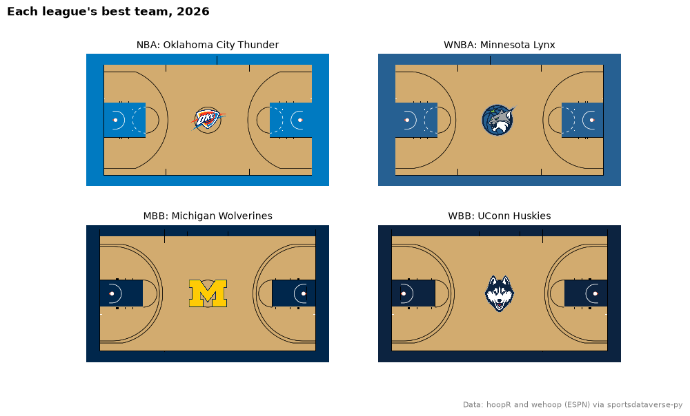
NBA, WNBA and college courts differ in their lines (the three-point arc, the lane width), and sportypy draws each league's own. Each court here belongs to its league's best team: the most regular-season wins for the pros, the highest adjusted efficiency margin in college.

def most_wins(box: pl.DataFrame) -> str:
    regular = box.filter(pl.col("season_type") == 2)
    wins = regular.group_by("team_abbreviation").agg(pl.col("team_winner").sum())
    return wins.sort(["team_winner", "team_abbreviation"], descending=[True, False])["team_abbreviation"][0]


def top_rated(ratings: pl.DataFrame) -> str:
    return ratings.sort("adj_em", descending=True)["team_id"][0]


courts = [
    ("nba", most_wins(nba.load_nba_team_boxscore(seasons=[SEASON]))),
    ("wnba", most_wins(wnba.load_wnba_team_boxscore(seasons=[SEASON]))),
    ("mbb", top_rated(mbb.load_mbb_ratings(SEASON))),
    ("wbb", top_rated(wbb.load_wbb_ratings(SEASON))),
]
fig, axes = plt.subplots(2, 2, figsize=(10, 6))
for ax, (league, team) in zip(axes.flat, courts, strict=True):
    sdvplot.surface(league, team, ax=ax, center_logo=0.3)
    name = sdvplot.teams(league).filter(pl.col("team_id") == sdvplot.resolve(team, league))["name"].item()
    ax.set_title(f"{league.upper()}: {name}", fontsize=10)
fig.suptitle("Each league's best team, 2026", x=0.01, ha="left", fontweight="bold")
fig.text(0.99, 0.01, "Data: hoopR and wehoop (ESPN) via sportsdataverse-py", ha="right", fontsize=8, color="grey")
plt.show()

4. An NBA shot chart from the stats-API frame

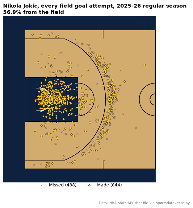
The stats API's shot locations (LOC_X / LOC_Y, x_legacy / y_legacy in sportsdataverse-py) are in tenths of a foot with the hoop at the origin. sportypy's court has its origin at center court, in feet. court_coords converts one to the other and adds court_x / court_y; every shot lands on the left half, so draw that half with display_range="defense". The shots come from the stats-API shot file the SportsDataverse publishes on GitHub, so nothing calls stats.nba.com. Nikola Jokic's season:

shots = nba.load_nba_stats_shots(seasons=SEASON - 1)  # this loader takes the season's start year
jokic = sdvplot.court_coords(shots.filter((pl.col("person_id") == 203999) & (pl.col("season_type_id") == "2")))
print(jokic.select("x_legacy", "y_legacy", "court_x", "court_y").head(3))
made, missed = jokic.filter(pl.col("shot_result") == "Made"), jokic.filter(pl.col("shot_result") == "Missed")

fig, ax = plt.subplots(figsize=(7.5, 7))
sdvplot.surface("nba", "DEN", ax=ax, display_range="defense")
ax.scatter(missed["court_x"], missed["court_y"], marker="x", s=14, linewidths=0.8, color="#3d3d3d", alpha=0.6,
           zorder=20, label=f"Missed ({missed.height})")  # fmt: skip
ax.scatter(made["court_x"], made["court_y"], s=18, color=sdvplot.team_colors("DEN", "nba", "secondary"),
           edgecolors="black", linewidths=0.4, zorder=21, label=f"Made ({made.height})")  # fmt: skip
ax.legend(loc="upper center", bbox_to_anchor=(0.5, 0.02), ncols=2, frameon=False)
ax.set_title(f"Nikola Jokic, every field goal attempt, 2025-26 regular season\n"
             f"{made.height / jokic.height:.1%} from the field", loc="left", fontweight="bold")  # fmt: skip
fig.text(0.99, 0.01, "Data: NBA stats API shot file via sportsdataverse-py", ha="right", fontsize=8, color="grey")
plt.show()

| x_legacy | y_legacy | court_x | court_y |
|----------|----------|---------|---------|
| 47       | 32       | -38.55  | 4.7     |
| 37       | 16       | -40.15  | 3.7     |
| -2       | 0        | -41.75  | -0.2    |

5. The same for the WNBA

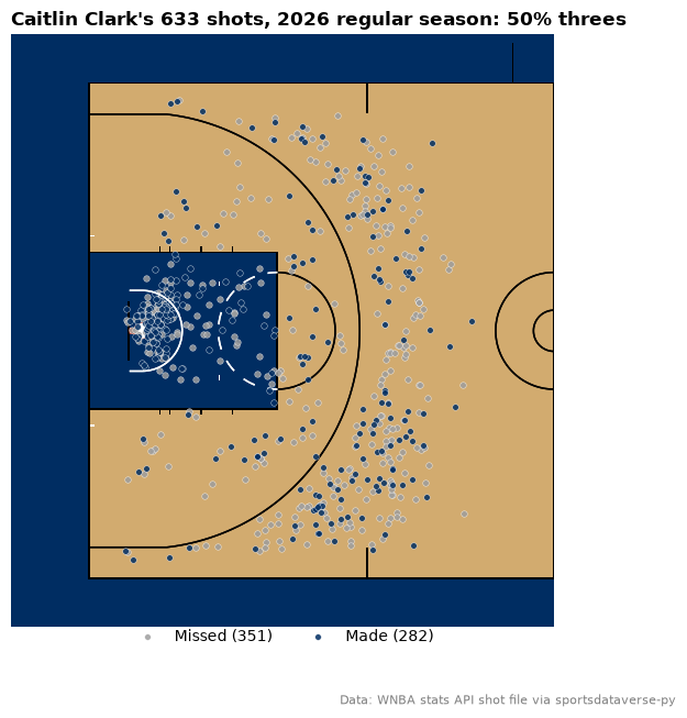
stats.wnba.com uses the same frame, so court_coords works unchanged; surface("wnba") draws the WNBA's court, whose three-point arc sits closer to the basket than the NBA's. The file has no season-type column, but the game id says it: 102... is the regular season, 104... the playoffs. Caitlin Clark's 2026 regular season:

clark = sdvplot.court_coords(
    wnba.load_wnba_stats_shots(seasons=SEASON).filter(
        (pl.col("person_id") == 1642286) & pl.col("game_id").str.starts_with("102")  # 102: regular season
    )
).with_columns(three=pl.col("shot_value") == 3)
colors = {"Made": sdvplot.team_colors("IND", "wnba"), "Missed": "#9e9e9e"}

fig, ax = plt.subplots(figsize=(7.5, 7))
sdvplot.surface("wnba", "IND", ax=ax, display_range="defense")
for result in ("Missed", "Made"):
    group = clark.filter(pl.col("shot_result") == result)
    ax.scatter(group["court_x"], group["court_y"], s=16, color=colors[result], edgecolors="white",
               linewidths=0.3, alpha=0.85, zorder=20, label=f"{result} ({group.height})")  # fmt: skip
threes = clark.filter(pl.col("three"))
ax.legend(loc="upper center", bbox_to_anchor=(0.5, 0.02), ncols=2, frameon=False)
ax.set_title(f"Caitlin Clark's {clark.height} shots, 2026 regular season: {threes.height / clark.height:.0%} threes",
             loc="left", fontweight="bold")  # fmt: skip
fig.text(0.99, 0.01, "Data: WNBA stats API shot file via sportsdataverse-py", ha="right", fontsize=8, color="grey")
plt.show()

6. A vertical half court: rotate the surface and the data

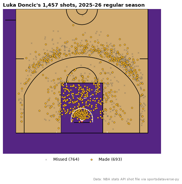
sportypy's rotation= turns the drawing; turn the points the same way. A quarter turn counterclockwise (rotation=90) maps each point (x, y) to (-y, x) and puts the basket at the bottom, the way many shot charts are drawn. display_range still names the half of the unrotated court. Luka Doncic's shots, made in the Lakers' gold:

luka = sdvplot.court_coords(shots.filter((pl.col("person_id") == 1629029) & (pl.col("season_type_id") == "2")))
luka = luka.with_columns(x=-pl.col("court_y"), y=pl.col("court_x"))  # (x, y) -> (-y, x): a quarter turn
made, missed = luka.filter(pl.col("shot_result") == "Made"), luka.filter(pl.col("shot_result") == "Missed")

fig, ax = plt.subplots(figsize=(7, 7))
sdvplot.surface("nba", "LAL", ax=ax, rotation=90, display_range="defense")
ax.scatter(missed["x"], missed["y"], marker="x", s=12, linewidths=0.7, color="#555555", alpha=0.5, zorder=20,
           label=f"Missed ({missed.height})")  # fmt: skip
ax.scatter(made["x"], made["y"], s=16, color=sdvplot.team_colors("LAL", "nba", "secondary"), edgecolors="black",
           linewidths=0.4, zorder=21, label=f"Made ({made.height})")  # fmt: skip
ax.legend(loc="upper center", bbox_to_anchor=(0.5, 0.0), ncols=2, frameon=False)
ax.set_title(f"Luka Doncic's {luka.height:,} shots, 2025-26 regular season", loc="left", fontweight="bold")
fig.text(0.99, 0.01, "Data: NBA stats API shot file via sportsdataverse-py", ha="right", fontsize=8, color="grey")
plt.show()

7. A hockey goal map on a team-colored rink

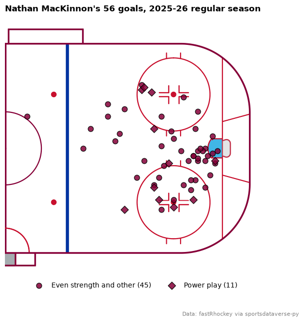
fastRhockey's x_fixed / y_fixed are in feet on the NHL rink's frame, the same one sportypy draws, with the home team shooting right. Mirror the away goals (flip both signs) to put every goal at one net, then draw the attacking half with display_range="offense". Nathan MacKinnon's regular-season goals:

pbp = nhl.load_nhl_pbp_lite(seasons=[SEASON]).select(
    "event_type", "event_player_1_name", "season_type", "strength_state", "x_fixed", "y_fixed"
)
goals = pbp.filter(
    (pl.col("event_player_1_name") == "Nathan MacKinnon")
    & (pl.col("event_type") == "GOAL")
    & (pl.col("season_type") == "R")
).with_columns(
    x=pl.col("x_fixed").abs(),
    y=pl.when(pl.col("x_fixed") < 0).then(-pl.col("y_fixed")).otherwise(pl.col("y_fixed")),
    power_play=pl.col("strength_state").is_in(["5v4", "5v3", "4v3"]),
)
fig, ax = plt.subplots(figsize=(7, 7))
sdvplot.surface("nhl", "COL", ax=ax, display_range="offense")
for pp, label, marker in [(False, "Even strength and other", "o"), (True, "Power play", "D")]:
    g = goals.filter(pl.col("power_play") == pp)
    ax.scatter(g["x"], g["y"], marker=marker, s=60, color=sdvplot.team_colors("COL", "nhl"),
               edgecolors="black", alpha=0.85, zorder=30, label=f"{label} ({g.height})")  # fmt: skip
ax.legend(loc="upper center", bbox_to_anchor=(0.5, 0.02), ncols=2, frameon=False)
ax.set_title(f"Nathan MacKinnon's {goals.height} goals, 2025-26 regular season", loc="left", fontweight="bold")
fig.text(0.99, 0.01, "Data: fastRhockey via sportsdataverse-py", ha="right", fontsize=8, color="grey")
plt.show()

8. A baseball field with a logo in center field

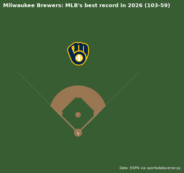
Baseball fields have no team-colored lines, and the field's origin is home plate, so center_logo would put the logo on the plate. Draw the field, then place the logo yourself with add_logos: here in center field, for the team with MLB's best 2026 record (ESPN's final standings).

import sportsdataverse.mlb as mlb

best = mlb.espn_mlb_standings(season=SEASON).sort("win_percent", descending=True).row(0, named=True)
ax = sdvplot.surface("mlb")
ax.figure.set_size_inches(7, 6)
sdvplot.add_logos(ax, [0], [260], [best["team_abbreviation"]], league="mlb", height=0.18, zorder=40)
ax.set_title(f"{best['team_display_name']}: MLB's best record in {SEASON} ({best['wins']:.0f}-{best['losses']:.0f})",
             loc="left", fontweight="bold", color="white")  # fmt: skip
ax.figure.text(0.98, 0.02, "Data: ESPN via sportsdataverse-py", ha="right", fontsize=8, color="white")
plt.show()

9. A soccer shot map on an mplsoccer pitch

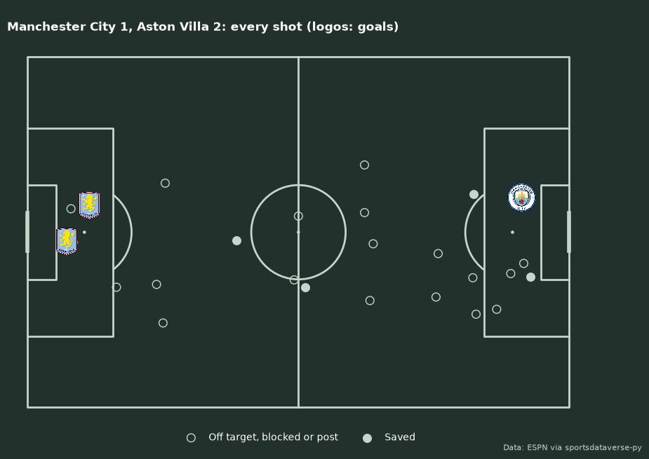
For soccer, mplsoccer draws the pitch and sdvplot's logos go on its matplotlib Axes. ESPN's play-by-play gives each shot's position as fractions of the pitch: field_position_x measured from the goal the team attacks, field_position_y across. The home team shoots right, the away team left; goals are the scorer's logo. The Premier League's final day of 2025-26, Manchester City against Aston Villa (ESPN team ids 382 and 362):

from mplsoccer import Pitch

EVENT, HOME, AWAY = 740970, "382", "362"
plays = soccer.espn_soccer_game_plays("eng.1", EVENT, cid=EVENT)
shots = (
    plays.filter(pl.col("type_text").str.contains("(?i)shot|goal") & (pl.col("type_text") != "Assists Shot"))
    .with_columns(team=pl.col("team_$ref").str.extract(r"/teams/(\d+)"))
    .with_columns(
        x=pl.when(pl.col("team") == HOME)
        .then((1 - pl.col("field_position_x")) * 105)
        .otherwise(pl.col("field_position_x") * 105),
        y=pl.col("field_position_y") * 68,
    )
)
goals = shots.filter(pl.col("scoring_play"))
on_target = shots.filter(pl.col("type_text") == "Shot On Target")
other = shots.filter(~pl.col("scoring_play") & (pl.col("type_text") != "Shot On Target"))

pitch = Pitch(pitch_type="custom", pitch_length=105, pitch_width=68, pitch_color="#22312b", line_color="#c7d5cc")
fig, ax = pitch.draw(figsize=(10, 6.5))
pitch.scatter(other["x"], other["y"], s=70, facecolors="none", edgecolors="#c7d5cc", ax=ax,
              label="Off target, blocked or post")  # fmt: skip
pitch.scatter(on_target["x"], on_target["y"], s=70, color="#c7d5cc", ax=ax, label="Saved")
sdvplot.add_logos(ax, goals["x"], goals["y"], goals["team"], league="soccer", height=0.08, zorder=5)
sdvplot.add_logos(ax, [8, 97], [74, 74], [AWAY, HOME], league="soccer", height=0.1, zorder=5)
ax.legend(loc="lower center", bbox_to_anchor=(0.5, -0.06), ncols=2, frameon=False, labelcolor="white")
home_goals = goals.filter(pl.col("team") == HOME).height
ax.set_title(f"Manchester City {home_goals}, Aston Villa {goals.height - home_goals}: every shot (logos: goals)",
             color="white", fontweight="bold", loc="left")  # fmt: skip
fig.set_facecolor("#22312b")
fig.text(0.99, 0.01, "Data: ESPN via sportsdataverse-py", ha="right", fontsize=8, color="#c7d5cc")
plt.show()

Run it yourself

Download the notebook (outputs cleared) or open it on GitHub.