College football

Nine charts and tables from the 2025 college football season: all 136 FBS teams on one scatter, conference small multiples, a conference standings table, the national champion's season, a rivalry, FCS upsets, an interactive Altair chart, a ranked bar chart and a tier list. The data comes from the cfbfastR releases and ESPN through sportsdataverse.cfb.

import matplotlib.pyplot as plt
import polars as pl
import sportsdataverse.cfb as cfb

import sdvplot

SEASON = 2025
CAPTION = f"Data: cfbfastR via sportsdataverse-py | {SEASON} season"

# sdvplot team ids are strings: cast the loaders' integer ESPN ids once, here
summaries = cfb.load_cfb_team_summaries([SEASON]).select(
    pl.col("team_id").cast(pl.Utf8), "pos_team", "conference", "EPAplay_off", "EPAplay_def"
)
schedule = cfb.load_cfb_schedule([SEASON]).with_columns(pl.col("home_id", "away_id").cast(pl.Utf8))
names = sdvplot.teams("cfb").select("team_id", school="short_name")
summaries.height, schedule.height

(136, 3831)

1. All 136 FBS teams on one chart

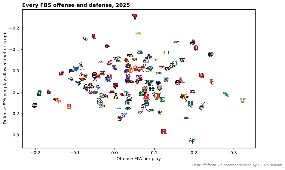
Offensive EPA per play against defensive EPA per play allowed, from the cfbfastR team summaries. With this many teams the logos have to be small: height=0.045 makes each one 4.5% of the plot's height.

fig, ax = plt.subplots(figsize=(10, 6))
ax.axvline(summaries["EPAplay_off"].mean(), color="grey", lw=0.8, ls="--")
ax.axhline(summaries["EPAplay_def"].mean(), color="grey", lw=0.8, ls="--")
ax.scatter(summaries["EPAplay_off"], summaries["EPAplay_def"], s=0)
ax.margins(0.06)
sdvplot.add_logos(
    ax,
    summaries["EPAplay_off"],
    summaries["EPAplay_def"],
    summaries["team_id"],
    league="cfb",
    season=SEASON,
    height=0.045,
)
ax.invert_yaxis()
ax.set(xlabel="Offense EPA per play", ylabel="Defense EPA per play allowed (better is up)")
ax.set_title(f"Every FBS offense and defense, {SEASON}", loc="left", fontweight="bold")
fig.text(0.99, 0.01, CAPTION, ha="right", fontsize=8, color="grey")
plt.show()

2. Conference small multiples with plotnine

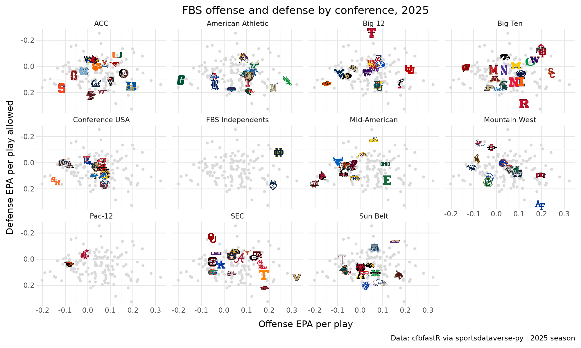
The same data, one panel per conference: every FBS team as a grey dot behind, the conference's own teams as logos. The grey layer gets a copy of the data without the conference column, so plotnine repeats it in every panel.

from plotnine import aes, facet_wrap, geom_point, ggplot, labs, scale_y_reverse, theme, theme_minimal

from sdvplot.plotnine import geom_sdv_logos

(
    ggplot(summaries.to_pandas(), aes("EPAplay_off", "EPAplay_def"))
    + geom_point(data=summaries.drop("conference").to_pandas(), color="#d9d9d9", size=1)
    + geom_sdv_logos(aes(team="team_id"), league="cfb", season=SEASON, height=0.13)
    + facet_wrap("conference", ncol=4)
    + scale_y_reverse()
    + labs(
        x="Offense EPA per play",
        y="Defense EPA per play allowed",
        title=f"FBS offense and defense by conference, {SEASON}",
        caption=CAPTION,
    )
    + theme_minimal()
    + theme(figure_size=(10, 6))
)

3. A conference standings table

Big Ten records built from the schedule: conference games and all games through the regular season (the title game and bowls left out). gt_sdv_logos turns the id column into logos and gt_fmt_tally writes each pair of win and loss columns as one record.

from great_tables import GT

from sdvplot.great_tables import gt_fmt_tally, gt_sdv_logos, gt_theme_athletic

regular = schedule.filter(pl.col("completed"), pl.col("season_type") == "regular", pl.col("week") <= 14)
sides = pl.concat(
    [
        regular.select(
            "conference_game", team_id="home_id", conf="home_conference", pf="home_points", pa="away_points"
        ),
        regular.select(
            "conference_game", team_id="away_id", conf="away_conference", pf="away_points", pa="home_points"
        ),
    ]
).with_columns(win=pl.col("pf") > pl.col("pa"))

big_ten = (
    sides.filter(pl.col("conf") == "Big Ten")
    .group_by("team_id")
    .agg(
        conf_w=(pl.col("win") & pl.col("conference_game")).sum(),
        conf_l=(~pl.col("win") & pl.col("conference_game")).sum(),
        w=pl.col("win").sum(),
        l=(~pl.col("win")).sum(),
        pf=pl.col("pf").sum(),
        pa=pl.col("pa").sum(),
    )
    .join(names, on="team_id")
    .sort(["conf_w", "w", "pf"], descending=True)
    .select("team_id", "school", "conf_w", "conf_l", "w", "l", "pf", "pa")
)

(
    GT(big_ten)
    .pipe(gt_sdv_logos, "team_id", league="cfb", season=SEASON, height=24)
    .pipe(gt_fmt_tally, ["conf_w", "conf_l"], label="Conf")
    .pipe(gt_fmt_tally, ["w", "l"], label="Overall")
    .cols_label(team_id="", school="", pf="PF", pa="PA")
    .tab_header(title=f"Big Ten standings, {SEASON}", subtitle="Regular season, before the title game")
    .tab_source_note(CAPTION)
    .pipe(gt_theme_athletic, density="compact")
)

4. The national champion's season, with a logo in the title

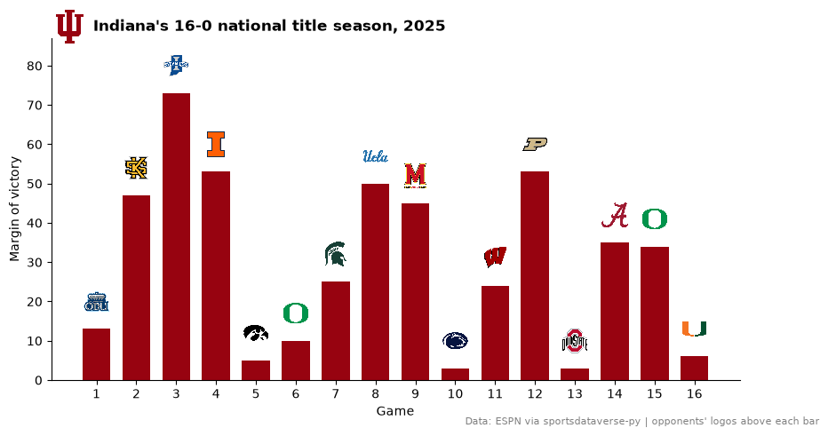
Indiana went 16-0. Each bar is one game's margin in Indiana's primary color, the opponent's logo above it, and title_image puts the Indiana logo beside the title. resolve turns the school name into its id.

from sdvplot.matplotlib import title_image

team = sdvplot.resolve("Indiana", "cfb")
games = (
    schedule.filter(pl.col("completed"), (pl.col("home_id") == team) | (pl.col("away_id") == team))
    .sort("start_date")
    .with_columns(
        home=pl.col("home_id") == team,
        opponent=pl.when(pl.col("home_id") == team).then("away_id").otherwise("home_id"),
    )
    .with_columns(
        margin=pl.when(pl.col("home"))
        .then(pl.col("home_points") - pl.col("away_points"))
        .otherwise(pl.col("away_points") - pl.col("home_points"))
    )
)
game_no = list(range(1, games.height + 1))

fig, ax = plt.subplots(figsize=(10, 5))
ax.bar(game_no, games["margin"], color=sdvplot.team_colors(team, "cfb"), width=0.7)
sdvplot.add_logos(ax, game_no, games["margin"] + 7, games["opponent"], league="cfb", season=SEASON, height=0.08)
ax.set_ylim(0, games["margin"].max() + 14)
ax.set_xticks(game_no)
ax.set(xlabel="Game", ylabel="Margin of victory")
ax.spines[["top", "right"]].set_visible(False)
record = f"{(games['margin'] > 0).sum()}-{(games['margin'] < 0).sum()}"
title_image(
    ax,
    team,
    f"Indiana's {record} national title season, {SEASON}",
    league="cfb",
    season=SEASON,
    height=30,
    loc="left",
    fontweight="bold",
)
fig.text(
    0.99,
    0.01,
    "Data: ESPN via sportsdataverse-py | opponents' logos above each bar",
    ha="right",
    fontsize=8,
    color="grey",
)
plt.show()

5. A rivalry, season by season

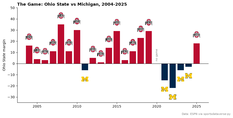
Ohio State against Michigan since 2004 (load_cfb_schedule for 22 seasons). Each bar is the margin from Ohio State's side, colored for the winner, with the winner's logo at the end of the bar.

osu, mich = sdvplot.resolve(["Ohio State", "Michigan"], "cfb")
history = cfb.load_cfb_schedule(list(range(2004, SEASON + 1))).with_columns(pl.col("home_id", "away_id").cast(pl.Utf8))
rivalry = (
    history.filter(pl.col("home_id").is_in([osu, mich]), pl.col("away_id").is_in([osu, mich]), pl.col("completed"))
    .with_columns(
        osu_margin=pl.when(pl.col("home_id") == osu)
        .then(pl.col("home_points") - pl.col("away_points"))
        .otherwise(pl.col("away_points") - pl.col("home_points"))
    )
    .with_columns(winner=pl.when(pl.col("osu_margin") > 0).then(pl.lit(osu)).otherwise(pl.lit(mich)))
    .sort("season")
)

fig, ax = plt.subplots(figsize=(10, 5))
ax.bar(rivalry["season"], rivalry["osu_margin"], color=sdvplot.team_colors(rivalry["winner"], "cfb").to_list())
tip = rivalry["osu_margin"] + pl.Series([8 if m > 0 else -8 for m in rivalry["osu_margin"]])
sdvplot.add_logos(ax, rivalry["season"], tip, rivalry["winner"], league="cfb", season=SEASON, height=0.08)
ax.axhline(0, color="black", lw=0.8)
ax.text(2020, 2, "no game", ha="center", fontsize=8, color="grey", rotation=90, va="bottom")
ax.set_ylim(-35, 50)
ax.set(ylabel="Ohio State margin")
ax.spines[["top", "right"]].set_visible(False)
ax.set_title("The Game: Ohio State vs Michigan, 2004-2025", loc="left", fontweight="bold")
fig.text(0.99, 0.01, "Data: ESPN via sportsdataverse-py", ha="right", fontsize=8, color="grey")
plt.show()

6. FBS, FCS and the schools sdvplot does not know

The index has every FBS and FCS program and most of Division II and III. The 2025 schedule also lists opponents outside the NCAA divisions (NAIA schools, mostly); most of those do not resolve, and sdvplot says so in one warning instead of guessing.

import warnings

opponents = pl.concat(
    [
        schedule.select(team_id="home_id", division="home_division"),
        schedule.select(team_id="away_id", division="away_division"),
    ]
).unique("team_id", maintain_order=True)

with warnings.catch_warnings(record=True) as caught:
    warnings.simplefilter("always")
    resolved = sdvplot.resolve(opponents["team_id"], "cfb")
print(str(caught[0].message)[:160], "...")

(
    opponents.with_columns(found=resolved.is_not_null())
    .group_by("division")
    .agg(teams=pl.len(), in_sdvplot=pl.col("found").sum())
    .sort("teams", descending=True)
)

33 value(s) did not resolve to a cfb team: '15' (unknown), '2366' (unknown), '127991' (unknown), '110254' (unknown), '2395' (unknown), '2939' (unknown), '108358 ...

division	teams	in_sdvplot
iii	240	237
ii	162	158
fbs	136	136
fcs	129	129
null	32	6

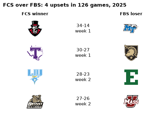
FCS teams have their own logos and colors, so an FCS-over-FBS upset draws like any other game. In 2025 the FCS won four of its games against FBS teams:

cross = schedule.filter(
    pl.col("completed"),
    pl.concat_list("home_division", "away_division").list.sort() == ["fbs", "fcs"],
)
fcs_home = pl.col("home_division") == "fcs"
upsets = cross.filter(pl.when(fcs_home).then("home_winner").otherwise("away_winner")).select(
    winner=pl.when(fcs_home).then("home_id").otherwise("away_id"),
    loser=pl.when(fcs_home).then("away_id").otherwise("home_id"),
    score=pl.format(
        "{}-{}", pl.max_horizontal("home_points", "away_points"), pl.min_horizontal("home_points", "away_points")
    ),
    week="week",
)

rows = list(range(upsets.height, 0, -1))
fig, ax = plt.subplots(figsize=(7, 4.5))
ax.set(xlim=(0, 1), ylim=(0.4, upsets.height + 0.6))
ax.axis("off")
sdvplot.add_logos(ax, [0.2] * upsets.height, rows, upsets["winner"], league="cfb", season=SEASON, height=0.17)
sdvplot.add_logos(ax, [0.8] * upsets.height, rows, upsets["loser"], league="cfb", season=SEASON, height=0.17)
for y, row in zip(rows, upsets.iter_rows(named=True), strict=True):
    ax.text(0.5, y, f"{row['score']}\nweek {row['week']}", ha="center", va="center", fontsize=11)
ax.text(0.2, upsets.height + 0.55, "FCS winner", ha="center", fontweight="bold")
ax.text(0.8, upsets.height + 0.55, "FBS loser", ha="center", fontweight="bold")
ax.set_title(
    f"FCS over FBS: {upsets.height} upsets in {cross.height} games, {SEASON}", loc="left", fontweight="bold", pad=18
)
plt.show()

7. An interactive Altair chart

The cfbfastR opponent-adjusted ratings (load_cfb_ratings) as an Altair chart with tooltips. add_logos layers the logos onto the chart; the transparent points underneath carry the tooltips.

import altair as alt

ratings = (
    cfb.load_cfb_ratings([SEASON])
    .with_columns(pl.col("team_id").cast(pl.Utf8))
    .join(names, on="team_id")
    .select("team_id", "school", "adj_off_epa", "adj_def_epa", "adj_net", "net_rank")
)

points = (
    alt.Chart(ratings.to_pandas())
    .mark_circle(size=250, opacity=0)
    .encode(
        x=alt.X("adj_off_epa", title="Adjusted offense EPA per play"),
        y=alt.Y("adj_def_epa", title="Adjusted defense EPA per play (better is up)", scale=alt.Scale(reverse=True)),
        tooltip=["school", "net_rank", alt.Tooltip("adj_net", format=".3f")],
    )
    .properties(width=640, height=440, title=f"Opponent-adjusted FBS ratings, {SEASON}")
)
sdvplot.add_logos(
    points, ratings["adj_off_epa"], ratings["adj_def_epa"], ratings["team_id"], league="cfb", season=SEASON, height=0.05
)

8. A ranked bar chart with logos on the y axis

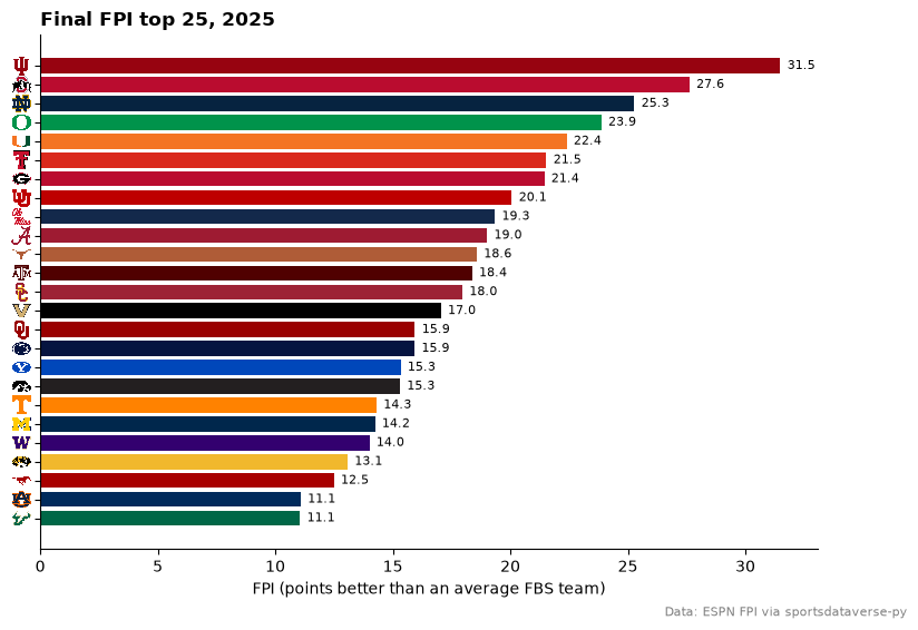
ESPN's final 2025 FPI (load_cfb_fpi_weekly, the snapshot after the title game), top 25. The bars use the teams' ESPN colors and axis_logos(ax, "y") replaces the team ids on the axis.

fpi = cfb.load_cfb_fpi_weekly([SEASON]).filter(pl.col("season_type") == 3)
top = (
    fpi.select(pl.col("team_id").cast(pl.Utf8), "fpi")
    .sort("fpi", descending=True)
    .head(25)
    .reverse()  # barh draws from the bottom up, so number one ends on top
)

fig, ax = plt.subplots(figsize=(9, 6))
ax.barh(top["team_id"], top["fpi"], color=sdvplot.team_colors(top["team_id"], "cfb").to_list())
for y, value in enumerate(top["fpi"]):
    ax.text(value + 0.3, y, f"{value:.1f}", va="center", fontsize=8)
sdvplot.axis_logos(ax, "y", league="cfb", season=SEASON, height=0.04)
ax.spines[["top", "right"]].set_visible(False)
ax.set_xlabel("FPI (points better than an average FBS team)")
ax.set_title(f"Final FPI top 25, {SEASON}", loc="left", fontweight="bold")
fig.text(0.99, 0.01, "Data: ESPN FPI via sportsdataverse-py", ha="right", fontsize=8, color="grey")
plt.show()

9. Tiers of a ranking you compute

A composite ranking: the average of each team's rank in two systems, cfbfastR's adjusted net EPA and FEI. The top 32 go into five tiers with team_tiers.

from sdvplot.matplotlib import team_tiers

composite = (
    cfb.load_cfb_ratings([SEASON])
    .with_columns(pl.col("team_id").cast(pl.Utf8), score=(pl.col("net_rank") + pl.col("fei_net_rank")) / 2)
    .sort("score")
    .head(32)
)
sizes = [4, 6, 7, 7, 8]  # teams per tier, top to bottom
composite = composite.with_columns(tier_no=pl.Series([tier for tier, n in enumerate(sizes, start=1) for _ in range(n)]))

fig = team_tiers(
    composite.select("tier_no", team="team_id"),
    "cfb",
    title=f"College football tiers, {SEASON}",
    subtitle="average rank in adjusted net EPA and FEI",
    caption=CAPTION,
    alpha=1,
    tier_desc={1: "Elite", 2: "Contenders", 3: "Very good", 4: "Good", 5: "Solid"},
)
plt.show()

Run it yourself

Download the notebook (outputs cleared) or open it on GitHub.