Soccer

Ten charts and tables from the 2025-26 Premier League, the 2025 MLS and NWSL seasons and the 2025-26 Champions League: a league table with crests, points against goal difference, every club's form in its own colors, a season of shots on a pitch, a lineup card, and MLS beside the NWSL. The data is ESPN's soccer feed, read through sportsdataverse-py (sportsdataverse.soccer), whose wrappers take ESPN's competition slug: eng.1 is the Premier League, usa.1 MLS, usa.nwsl the NWSL and uefa.champions the Champions League. The pitch examples need the surfaces extra (pip install "sdvplot[surfaces]").

import warnings

import matplotlib.pyplot as plt
import polars as pl
import sportsdataverse.soccer as soccer

import sdvplot

SEASON = 2025  # ESPN names a season by the year it starts: 2025 is the 2025-26 Premier League, and MLS/NWSL 2025

Load the Premier League once: the final table, and every club's 38 league matches from its ESPN schedule. The schedule payload also carries the club's color, which the charts below use. The points rebuilt from the results match the official table for all twenty clubs.

table = (
    soccer.espn_soccer_standings("eng.1", season=SEASON)
    .sort("rank")
    .with_columns(
        pl.col(
            "rank",
            "points",
            "games_played",
            "wins",
            "ties",
            "losses",
            "points_for",
            "points_against",
            "point_differential",
        ).cast(pl.Int64)
    )
)
rows, club_colors = [], {}
for team_id in table["team_id"]:
    raw = soccer.espn_soccer_team_schedule("eng.1", team_id=team_id, season=SEASON, return_parsed=False)
    club_colors[team_id] = "#" + raw["team"]["color"]
    for event in raw["events"]:
        us, them = sorted(event["competitions"][0]["competitors"], key=lambda c: c["id"] != team_id)
        rows.append(
            {
                "team_id": team_id,
                "event_id": event["id"],
                "date": event["date"][:10],
                "home_away": us["homeAway"],
                "opponent_id": them["id"],
                "gf": int(us["score"]["value"]),
                "ga": int(them["score"]["value"]),
            }
        )
games = (
    pl.DataFrame(rows)
    .sort("team_id", "date")
    .with_columns(
        pts=pl.when(pl.col("gf") > pl.col("ga")).then(3).when(pl.col("gf") == pl.col("ga")).then(1).otherwise(0),
        match=pl.int_range(1, pl.len() + 1).over("team_id"),
    )
)
check = games.group_by("team_id").agg(pl.col("pts").sum()).join(table.select("team_id", "points"), on="team_id")
assert (check["pts"] == check["points"]).all()
table.height, games.height

(20, 760)

1. One league key, thousands of clubs

sdvplot keeps every club ESPN covers under one league key, soccer: men's and women's clubs, youth sides and national teams from every competition. Names are not unique across that many clubs. "Arsenal" is both the men's club and Arsenal Women, so a name lookup refuses to guess: it returns None with one SdvplotWarning and suggest lists the candidates.

clubs = sdvplot.teams("soccer")
print(f"{clubs.height:,} clubs in the soccer index")
with warnings.catch_warnings(record=True) as caught:
    warnings.simplefilter("always")
    print(sdvplot.resolve(["Arsenal", "Liverpool", "Inter Miami CF"], "soccer"))
print(caught[0].message)
sdvplot.suggest("Arsenal", "soccer")

2,631 clubs in the soccer index
[None, None, '20232']
2 value(s) did not resolve to a soccer team: 'Arsenal' (ambiguous), 'Liverpool' (ambiguous). Use sdvplot.suggest() for candidates, or strict=True to raise.

[('19973', 'Arsenal'),
 ('359', 'Arsenal'),
 ('19299', 'Arsenal U21'),
 ('21823', 'Senegal'),
 ('654', 'Senegal')]

ESPN's team ids are the index's team_ids, so ids straight from the data resolve one to one, whatever the competition. Pass them, not names.

ids = sdvplot.resolve(table["team_id"], "soccer")
assert ids.to_list() == table["team_id"].to_list()
clubs.filter(pl.col("team_id").is_in(["359", "19973", "20232", "18206"])).select("team_id", "name")

team_id	name
18206	Orlando Pride
19973	Arsenal
20232	Inter Miami CF
359	Arsenal

2. Crests at any size

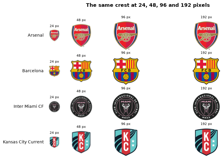
The soccer crests are 500-pixel PNGs, so logo_image(size=...) scales them down cleanly to anything from a table cell to a poster. size is the longest side in pixels.

sizes = [24, 48, 96, 192]
crests = {"359": "Arsenal", "83": "Barcelona", "20232": "Inter Miami CF", "20907": "Kansas City Current"}
fig, axes = plt.subplots(len(crests), len(sizes), figsize=(9, 6), gridspec_kw={"width_ratios": sizes})
for row, (team_id, name) in zip(axes, crests.items(), strict=True):
    for ax, size in zip(row, sizes, strict=True):
        img = sdvplot.logo_image(team_id, "soccer", size=size)
        ax.imshow(img)
        ax.set_title(f"{img.width} px", fontsize=8)
        ax.axis("off")
    row[0].text(-0.4, 0.5, name, transform=row[0].transAxes, ha="right", va="center", fontsize=10)
fig.suptitle("The same crest at 24, 48, 96 and 192 pixels", fontweight="bold")
plt.show()

3. The Premier League table with crests

A final table in the Premier League's own look: gt_sdv_logos turns the ESPN ids into crests, gt_theme_pl sets the league's purple, and gt_cutline marks the Champions League places and the drop. Form is each club's last five results, oldest first.

from great_tables import GT

from sdvplot.great_tables import gt_cutline, gt_sdv_logos, gt_theme_pl

form = (
    games.sort("date")
    .group_by("team_id", maintain_order=True)
    .agg(pl.col("pts").tail(5).replace_strict({3: "W", 1: "D", 0: "L"}, return_dtype=pl.String).str.join(" "))
    .rename({"pts": "form"})
)
pl_table = (
    table.join(form, on="team_id")
    .sort("rank")
    .select(  # a join does not keep row order
        "rank",
        pl.col("team_id").alias("crest"),
        "team",
        pl.col("games_played").alias("p"),
        pl.col("wins").alias("w"),
        pl.col("ties").alias("d"),
        pl.col("losses").alias("l"),
        pl.col("points_for").alias("gf"),
        pl.col("points_against").alias("ga"),
        pl.col("point_differential").alias("gd"),
        pl.col("points").alias("pts"),
        "form",
    )
)
gt = (
    GT(pl_table)
    .tab_header("Premier League 2025-26", "Final table")
    .cols_label(
        rank="", crest="", team="Club", p="P", w="W", d="D", l="L", gf="GF", ga="GA", gd="GD", pts="Pts", form="Last 5"
    )
    .fmt_number("gd", decimals=0, force_sign=True)
    .cols_align("left", ["team", "form"])
    .tab_source_note("Data: ESPN via sportsdataverse-py")
)
gt = gt_theme_pl(gt_sdv_logos(gt, "crest", league="soccer", height=22), density="compact")
gt = gt_cutline(gt, after=5, label="Champions League", label_position="above", color="#37003c")
gt_cutline(gt, after=17, label="Relegation", color="#37003c")

4. Points against goal difference

Goal difference explains most of a table, so a straight line through it shows who collected more or fewer points than their goals deserved. The crests are the points; the dashed line is the least-squares fit.

import numpy as np

slope, intercept = np.polyfit(table["point_differential"], table["points"], 1)
fig, ax = plt.subplots(figsize=(9, 6))
ax.scatter(table["point_differential"], table["points"], alpha=0)  # sets the limits; the crests are the points
xs = np.array([table["point_differential"].min() - 5, table["point_differential"].max() + 5])
ax.plot(xs, intercept + slope * xs, color="grey", lw=0.8, ls="--")
ax.margins(0.07)
sdvplot.add_logos(ax, table["point_differential"], table["points"], table["team_id"], league="soccer", height=0.07)
ax.set(xlabel="Goal difference", ylabel="Points")
ax.spines[["top", "right"]].set_visible(False)
ax.set_title("Premier League 2025-26: points against goal difference", loc="left", fontweight="bold", pad=20)
ax.text(
    0,
    1.015,
    f"Dashed line: the fit, {slope:.2f} points per goal of difference",
    transform=ax.transAxes,
    fontsize=9,
    color="grey",
)
fig.text(0.99, 0.01, "Data: ESPN via sportsdataverse-py", ha="right", fontsize=8, color="grey")
plt.show()

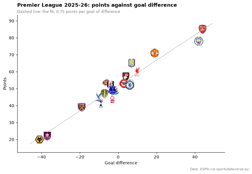
Aston Villa sit eight points above the line on 65 points from a +7 goal difference, Sunderland seven; Manchester City (78 points from +42) and Nottingham Forest finished about five below it.

5. Form, club by club, in club colors

Points from the last five matches across the season, one panel per club in final-table order. The index has no colors for soccer clubs yet (every row is color_source == "fallback", see the next example), so the lines use the color ESPN's schedule carried for each club. A few clubs' ESPN color is white; a dark line under each colored one keeps them all visible. geom_sdv_logos puts the crest in each panel.

from plotnine import (
    aes,
    element_blank,
    element_text,
    facet_wrap,
    geom_hline,
    geom_line,
    ggplot,
    labs,
    scale_color_manual,
    scale_x_continuous,
    scale_y_continuous,
    theme,
    theme_minimal,
)

from sdvplot.plotnine import geom_sdv_logos

order = table["team"].to_list()
names = table.select("team_id", "team")
rolling = (
    games.with_columns(form=pl.col("pts").rolling_sum(5).over("team_id"))
    .drop_nulls("form")
    .join(names, on="team_id")
    .to_pandas()
)
rolling["team"] = rolling["team"].astype("category").cat.set_categories(order)
crest_rows = names.with_columns(match=pl.lit(8), form=pl.lit(18.3)).to_pandas()  # above the lines (15 at most)
crest_rows["team"] = crest_rows["team"].astype("category").cat.set_categories(order)
(
    ggplot(rolling, aes("match", "form"))
    + geom_hline(yintercept=7.5, color="#cccccc", size=0.4)
    + geom_line(color="#222222", size=1.3)
    + geom_line(aes(color="team_id"), size=0.8, show_legend=False)
    + geom_sdv_logos(aes(team="team_id"), data=crest_rows, league="soccer", height=0.24)
    + scale_color_manual(values=club_colors)
    + scale_x_continuous(breaks=[5, 20, 38])
    + scale_y_continuous(breaks=[0, 5, 10, 15], limits=(0, 21))
    + facet_wrap("team", ncol=5)
    + labs(
        x="Match",
        y="Points from the last five matches",
        title="Premier League 2025-26: form across the season",
        caption="15 is five straight wins; the grey line, 7.5, is a point and a half a game. "
        "Data: ESPN via sportsdataverse-py",
    )
    + theme_minimal()
    + theme(
        figure_size=(10, 6),
        plot_title=element_text(weight="bold"),
        strip_text=element_text(size=8),
        panel_grid_minor=element_blank(),
    )
)

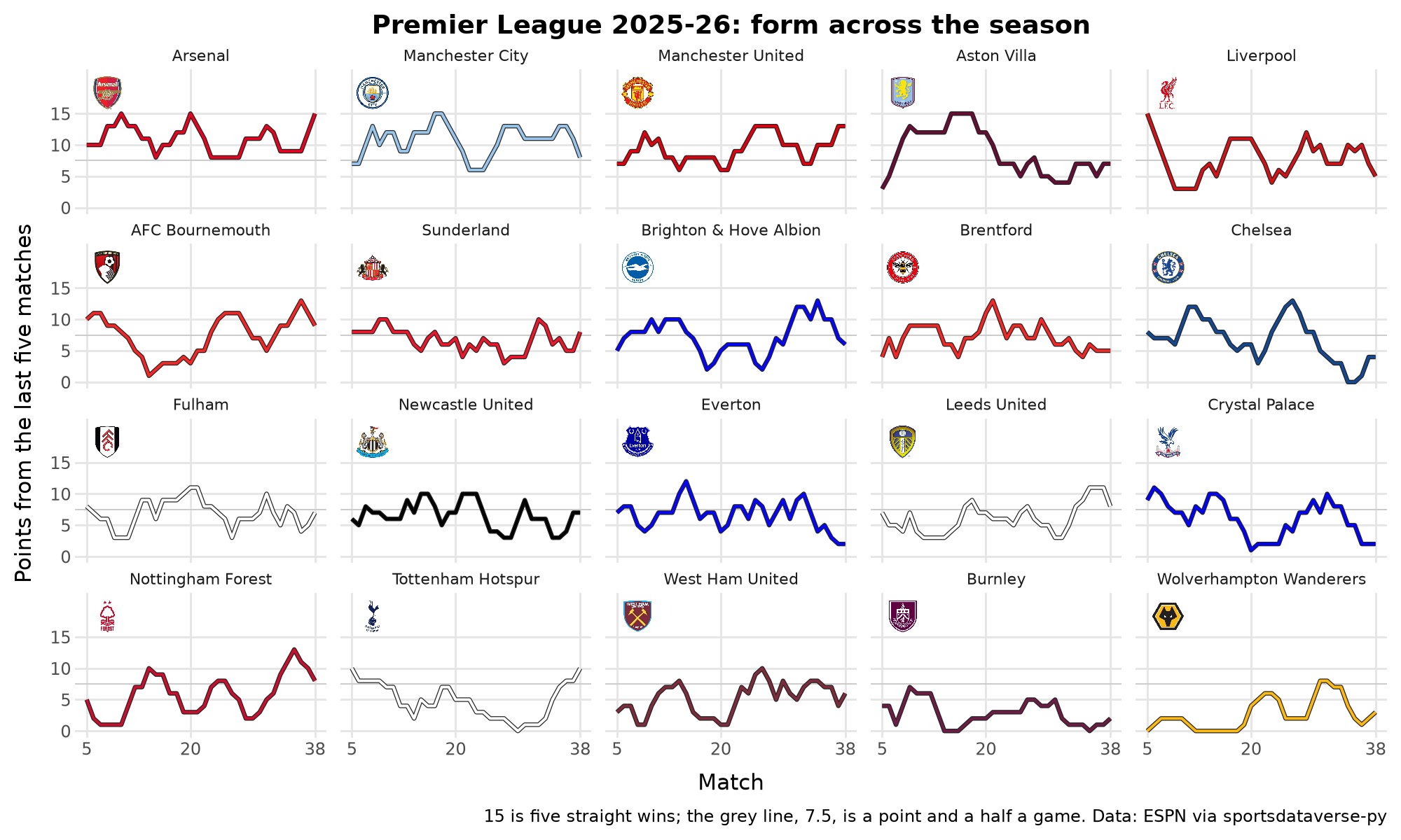
Arsenal ended the season on five straight wins; Aston Villa's run of 15 is an eight-match winning streak in November and December, and Chelsea lost six in a row in April and May.

6. Club colors for seaborn

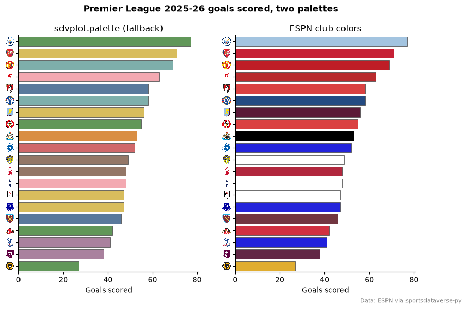
sdvplot.palette gives seaborn a {team: color} dict. For soccer those are the index's fallback colors: a colorblind-safe set that tells clubs apart but is not theirs. ESPN's own club colors identify the clubs, but six are shades of red and three are white. Both palettes, side by side, on goals scored; axis_logos swaps the team ids on the y axis for crests.

import seaborn as sns

print(sdvplot.teams("soccer")["color_source"].unique().to_list())
scored = table.sort("points_for", descending=True).select("team_id", "points_for").to_pandas()
fig, axes = plt.subplots(1, 2, figsize=(10, 6), sharex=True)
palettes = {
    "sdvplot.palette (fallback)": sdvplot.palette("soccer", teams=table["team_id"]),
    "ESPN club colors": club_colors,
}
for ax, (title, colors) in zip(axes, palettes.items(), strict=True):
    sns.barplot(
        scored,
        x="points_for",
        y="team_id",
        hue="team_id",
        palette=colors,
        legend=False,
        ax=ax,
        edgecolor="#555555",
        linewidth=0.6,
    )
    sdvplot.axis_logos(ax, "y", league="soccer", height=0.04)
    ax.set(title=title, xlabel="Goals scored", ylabel="")
    ax.spines[["top", "right"]].set_visible(False)
fig.suptitle("Premier League 2025-26 goals scored, two palettes", fontweight="bold")
fig.text(0.99, 0.01, "Data: ESPN via sportsdataverse-py", ha="right", fontsize=8, color="grey")
plt.show()

['fallback']

7. The champions' shots on a pitch

ESPN's match summaries carry a play-by-play commentary, and every shot in it has a location: fieldPositionX is the distance from the goal line as a fraction of half the pitch, fieldPositionY the position across it (below 0.5 is the shooter's left). surface("soccer") draws a FIFA pitch with sportypy; sized to 105 x 68 m and rotated so Arsenal attack upward, those fractions become meters. Shots without a recorded location (a few misses) are dropped, and own goals are left out because nobody on Arsenal shot them.

from sdvplot.matplotlib import title_image

SHOTS = ("shot-on-target", "shot-off-target", "shot-blocked", "shot-hit-woodwork")
GOALS = ("goal", "goal---header", "goal---volley", "goal---free-kick", "penalty---scored")
plays = []
for event_id in games.filter(pl.col("team_id") == "359")["event_id"]:
    summary = soccer.espn_soccer_summary("eng.1", event_id=event_id, return_parsed=False)
    # commentary plays name the team but carry no team id
    plays += [
        c["play"] for c in summary["commentary"] if c.get("play", {}).get("team", {}).get("displayName") == "Arsenal"
    ]
shots = (
    pl.DataFrame([{"type": p["type"]["type"], "fx": p["fieldPositionX"], "fy": p["fieldPositionY"]} for p in plays])
    .filter(pl.col("type").is_in(SHOTS + GOALS) & ((pl.col("fx") > 0) | (pl.col("fy") > 0)))
    .with_columns(x=(pl.col("fy") - 0.5) * 68, y=52.5 * (1 - pl.col("fx")), goal=pl.col("type").is_in(GOALS))
)
goals, misses = shots.filter(pl.col("goal")), shots.filter(~pl.col("goal"))

fig, ax = plt.subplots(figsize=(8, 5.8))
sdvplot.surface(
    "soccer", ax=ax, display_range="offense", rotation=90, pitch_updates={"pitch_length": 105, "pitch_width": 68}
)
ax.scatter(misses["x"], misses["y"], s=14, color="white", alpha=0.45, lw=0, zorder=20, label=f"Shots ({misses.height})")
ax.scatter(
    goals["x"],
    goals["y"],
    s=42,
    color=club_colors["359"],
    edgecolor="white",
    lw=0.7,
    zorder=21,
    label=f"Goals ({goals.height})",
)
ax.legend(loc="lower center", ncol=2, frameon=False, labelcolor="white", fontsize=10)
title_image(
    ax,
    "359",
    "Arsenal's 2025-26 Premier League shots",
    league="soccer",
    height=28,
    loc="left",
    fontweight="bold",
    pad=10,
)
ax.text(
    1,
    -0.02,
    "The champions' 38 league matches, own goals excluded. Data: ESPN via sportsdataverse-py",
    transform=ax.transAxes,
    ha="right",
    va="top",
    fontsize=8,
    color="grey",
)
plt.show()

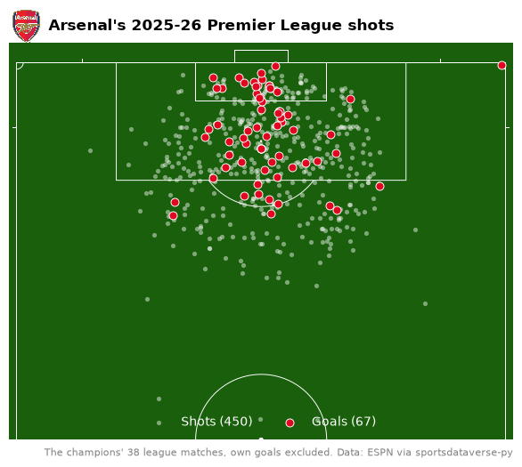
The goal alone in the top-right corner is where ESPN placed Noni Madueke's goal at Leeds, a shot "from a difficult angle and long range on the right": the locations are the data provider's, not computed.

8. A lineup card with mplsoccer

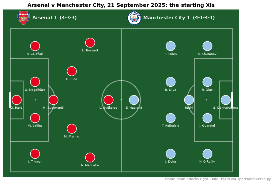
The same summaries carry both teams' starting XIs, the formation and each starter's formationPlace, which is Opta's position number. mplsoccer's formation() knows where each Opta number stands in each formation, so the card needs no hand-placed coordinates. Here is the title race's first meeting, Arsenal against Manchester City.

from mplsoccer import Pitch

arsenal_home = games.filter((pl.col("team_id") == "359") & (pl.col("home_away") == "home"))
event_id = arsenal_home.filter(pl.col("opponent_id") == "382")["event_id"].item()
summary = soccer.espn_soccer_summary("eng.1", event_id=event_id, return_parsed=False)
score = {t["team"]["id"]: t["score"] for t in summary["header"]["competitions"][0]["competitors"]}

pitch = Pitch(
    pitch_type="opta", pitch_color="#1d5c2c", line_color="white", line_alpha=0.5, pad_top=13, pad_left=5, pad_right=5
)
fig, ax = pitch.draw(figsize=(10, 6))
for side in summary["rosters"]:
    team_id = side["team"]["id"]
    xi = [p for p in side["roster"] if p.get("starter")]
    places = [int(p["formationPlace"]) for p in xi]
    shape = side["formation"].replace("-", "")
    away = side["homeAway"] == "away"
    pitch.formation(
        shape,
        positions=places,
        kind="scatter",
        flip=away,
        half=True,
        ax=ax,
        s=480,
        color=club_colors[team_id],
        edgecolor="white",
        lw=1.2,
        zorder=3,
    )
    pitch.formation(
        shape,
        positions=places,
        kind="text",
        flip=away,
        half=True,
        ax=ax,
        yoffset=-4.5,
        text=[p["athlete"]["shortName"] for p in xi],
        ha="center",
        va="top",
        fontsize=7.5,
        color="white",
        zorder=4,
    )
    left = 53 if away else 3
    sdvplot.add_logos(ax, [left + 3], [107], [team_id], league="soccer", height=0.09)
    ax.text(
        left + 7,
        107,
        f"{side['team']['displayName']} {score[team_id]}  ({side['formation']})",
        va="center",
        color="white",
        fontsize=11,
        fontweight="bold",
    )
ax.set_title("Arsenal v Manchester City, 21 September 2025: the starting XIs", fontweight="bold")
fig.text(0.99, 0.01, "Home team attacks right. Data: ESPN via sportsdataverse-py", ha="right", fontsize=8, color="grey")
plt.show()

9. MLS beside the NWSL

Both American leagues in one figure: goals scored and allowed per game, one facet per league. The clubs come from two competitions but the same soccer key, so one geom_sdv_logos layer draws them all; geom_mean_lines marks each league's averages, and the y axis is reversed so the good defenses sit at the top.

from plotnine import scale_y_reverse

from sdvplot.plotnine import geom_mean_lines

usa = pl.concat(
    [
        soccer.espn_soccer_standings(slug, season=SEASON).with_columns(league=pl.lit(name))
        for slug, name in [("usa.1", "MLS 2025"), ("usa.nwsl", "NWSL 2025")]
    ]
).with_columns(gf=pl.col("points_for") / pl.col("games_played"), ga=pl.col("points_against") / pl.col("games_played"))
(
    ggplot(usa.to_pandas(), aes("gf", "ga", x0="gf", y0="ga", team="team_id"))
    + geom_mean_lines(color="grey")
    + geom_sdv_logos(league="soccer", height=0.1)
    + scale_y_reverse()
    + facet_wrap("league", scales="free")
    + labs(
        x="Goals scored per game",
        y="Goals allowed per game (reversed)",
        title="Attack and defense in MLS and the NWSL, 2025 regular seasons",
        caption="Data: ESPN via sportsdataverse-py",
    )
    + theme_minimal()
    + theme(figure_size=(10, 5.5), plot_title=element_text(weight="bold"))
)

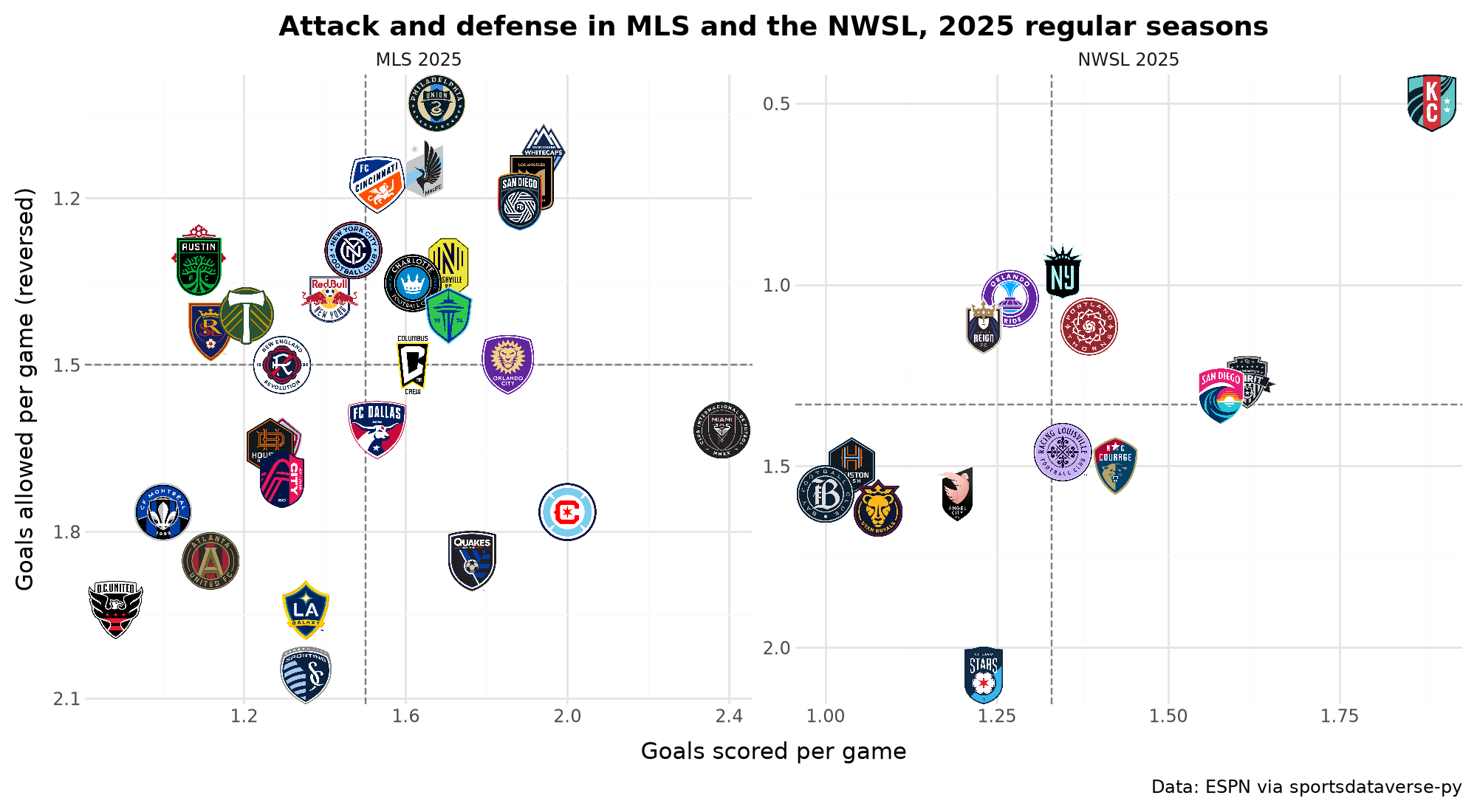
The Kansas City Current allowed half a goal a game, the best defense in either league by far; Inter Miami scored 2.38 a game, the most. MLS games averaged three goals, NWSL games 2.7.

10. Interactive: the Champions League league phase

Thirty-six clubs from fifteen countries, one league key: the 2025-26 Champions League league phase in Plotly, points against goal difference. Hover for the club and how it finished.

import plotly.graph_objects as go

ucl = soccer.espn_soccer_standings("uefa.champions", season=SEASON).with_columns(pl.col("note").fill_null("Eliminated"))
fig = go.Figure(
    go.Scatter(
        x=ucl["point_differential"],
        y=ucl["points"],
        mode="markers",
        marker={"opacity": 0},
        text=ucl["team"],
        customdata=ucl["note"],
        hovertemplate="%{text}<br>%{y} points, goal difference %{x:+}<br>%{customdata}<extra></extra>",
    )
)
fig = sdvplot.add_logos(fig, ucl["point_differential"], ucl["points"], ucl["team_id"], league="soccer", height=0.065)
fig.update_layout(
    title="Champions League 2025-26 league phase: points and goal difference",
    template="plotly_white",
    xaxis_title="Goal difference",
    yaxis_title="Points",
    width=800,
    height=560,
)
fig

Arsenal won all eight league-phase games; Kairat Almaty and Villarreal took one point each.

Run it yourself

Download the notebook (outputs cleared) or open it on GitHub.